knitr::opts_chunk$set(eval = F)Unsupervised Learning in R
Overview
Goal of unsupervised learning is to find structure in unlabeled data, vs. supervised learning’s goal is to make predictions based on labeled data (regression or classification). Finally, third type of ML is “reinforcement learning” which learns from feedback by operating in a real or synthetic environment.
Two major goals:
- “clustering” - find homogeneous subgroups within a population. Then we might label each subgroup.
- find patterns in features of data, e.g. like through dimensionality reduction, to achieve two goals:
visually represent high dimensional data
pre-processing step for supervised machine learning
k-means Clustering
k-means is a clustering algorithm
first assumes the number of subgroups (clusters) in data, then assigns each observation to one of these clusters
part of Base R:
kmeans(x, centers = 5, nstart = 20)has a random component
implies a downside: one single run may not find optimal solution; run multiple times to improve odds of finding best model
nstart: number of times it will be repeated
Example
image
# Create the k-means model: km.out
km.out <- kmeans(x, centers = 3, nstart = 20)

# Inspect the result
km.outK-means clustering with 3 clusters of sizes 52, 98, 150
Cluster means:
[,1] [,2]
1 0.6642455 -0.09132968
2 2.2171113 2.05110690
3 -5.0556758 1.96991743
Clustering vector:
[1] 2 2 2 2 2 2 2 2 2 2 2 2 1 2 2 2 2 1 1 2 2 2 2 2 2 2 2 2 2 2 2 2 2 2 2 2 1
[38] 1 1 2 2 2 2 1 2 2 2 2 2 2 2 2 2 2 2 2 2 2 1 2 2 2 2 2 2 2 2 2 2 2 2 2 2 1
[75] 2 2 2 2 2 2 2 2 2 2 2 2 2 2 2 2 2 2 2 2 2 2 2 2 2 2 3 3 3 3 3 3 3 3 3 3 3
[112] 3 3 3 3 3 3 3 3 3 3 3 3 3 3 3 3 3 3 3 3 3 3 3 3 3 3 3 3 3 3 3 3 3 3 3 3 3
[149] 3 3 3 3 3 3 3 3 3 3 3 3 3 3 3 3 3 3 3 3 3 3 3 3 3 3 3 3 3 3 3 3 3 3 3 3 3
[186] 3 3 3 3 3 3 3 3 3 3 3 3 3 3 3 3 3 3 3 3 3 3 3 3 3 3 3 3 3 3 3 3 3 3 3 3 3
[223] 3 3 3 3 3 3 3 3 3 3 3 3 3 3 3 3 3 3 3 3 3 3 3 3 3 3 3 3 1 1 1 1 2 1 1 1 1
[260] 1 1 1 1 1 1 1 1 1 1 1 1 1 1 1 1 2 2 1 1 2 1 1 1 1 1 1 2 1 1 1 1 1 1 2 1 1
[297] 1 2 1 1
Within cluster sum of squares by cluster:
[1] 95.50625 148.64781 295.16925
(between_SS / total_SS = 87.2 %)
Available components:
[1] "cluster" "centers" "totss" "withinss" "tot.withinss"
[6] "betweenss" "size" "iter" "ifault" summary(km.out)
Length Class Mode
cluster 300 -none- numeric
centers 6 -none- numeric
totss 1 -none- numeric
withinss 3 -none- numeric
tot.withinss 1 -none- numeric
betweenss 1 -none- numeric
size 3 -none- numeric
iter 1 -none- numeric
ifault 1 -none- numeric# Print the cluster membership component of the model
km.out$cluster
# Print the km.out object
print(km.out)output
# Print the cluster membership component of the model
km.out$cluster
  [1] 2 2 2 2 2 2 2 2 2 2 2 2 3 2 2 2 2 3 3 2 2 2 2 2 2 2 2 2 2 2 2 2 2 2 2 2 3
 [38] 3 3 2 2 2 2 3 2 2 2 2 2 2 2 2 2 2 2 2 2 2 3 2 2 2 2 2 2 2 2 2 2 2 2 2 2 3
 [75] 2 2 2 2 2 2 2 2 2 2 2 2 2 2 2 2 2 2 2 2 2 2 2 2 2 2 1 1 1 1 1 1 1 1 1 1 1
[112] 1 1 1 1 1 1 1 1 1 1 1 1 1 1 1 1 1 1 1 1 1 1 1 1 1 1 1 1 1 1 1 1 1 1 1 1 1
[149] 1 1 1 1 1 1 1 1 1 1 1 1 1 1 1 1 1 1 1 1 1 1 1 1 1 1 1 1 1 1 1 1 1 1 1 1 1
[186] 1 1 1 1 1 1 1 1 1 1 1 1 1 1 1 1 1 1 1 1 1 1 1 1 1 1 1 1 1 1 1 1 1 1 1 1 1
[223] 1 1 1 1 1 1 1 1 1 1 1 1 1 1 1 1 1 1 1 1 1 1 1 1 1 1 1 1 3 3 3 3 2 3 3 3 3
[260] 3 3 3 3 3 3 3 3 3 3 3 3 3 3 3 3 2 2 3 3 2 3 3 3 3 3 3 2 3 3 3 3 3 3 2 3 3
[297] 3 2 3 3
# Print the km.out object
print(km.out)
K-means clustering with 3 clusters of sizes 150, 98, 52

Cluster means:
        [,1]        [,2]
1 -5.0556758  1.96991743
2  2.2171113  2.05110690
3  0.6642455 -0.09132968

Clustering vector:
  [1] 2 2 2 2 2 2 2 2 2 2 2 2 3 2 2 2 2 3 3 2 2 2 2 2 2 2 2 2 2 2 2 2 2 2 2 2 3
 [38] 3 3 2 2 2 2 3 2 2 2 2 2 2 2 2 2 2 2 2 2 2 3 2 2 2 2 2 2 2 2 2 2 2 2 2 2 3
 [75] 2 2 2 2 2 2 2 2 2 2 2 2 2 2 2 2 2 2 2 2 2 2 2 2 2 2 1 1 1 1 1 1 1 1 1 1 1
[112] 1 1 1 1 1 1 1 1 1 1 1 1 1 1 1 1 1 1 1 1 1 1 1 1 1 1 1 1 1 1 1 1 1 1 1 1 1
[149] 1 1 1 1 1 1 1 1 1 1 1 1 1 1 1 1 1 1 1 1 1 1 1 1 1 1 1 1 1 1 1 1 1 1 1 1 1
[186] 1 1 1 1 1 1 1 1 1 1 1 1 1 1 1 1 1 1 1 1 1 1 1 1 1 1 1 1 1 1 1 1 1 1 1 1 1
[223] 1 1 1 1 1 1 1 1 1 1 1 1 1 1 1 1 1 1 1 1 1 1 1 1 1 1 1 1 3 3 3 3 2 3 3 3 3
[260] 3 3 3 3 3 3 3 3 3 3 3 3 3 3 3 3 2 2 3 3 2 3 3 3 3 3 3 2 3 3 3 3 3 3 2 3 3
[297] 3 2 3 3

Within cluster sum of squares by cluster:
[1] 295.16925 148.64781  95.50625
 (between_SS / total_SS =  87.2 %)

Available components:

[1] "cluster"      "centers"      "totss"        "withinss"     "tot.withinss"
[6] "betweenss"    "size"         "iter"         "ifault"
Take a look at all the different components of a k-means model object as you may need to access them in later exercises. Because printing the whole model object to the console outputs many different things, you may wish to instead print a specific component of the model object using the $ operator. Great work!
# Scatter plot of x
plot(x, col = km.out$cluster,
     main = "k-means with 3 clusters",
     xlab = "", ylab = "")
out
How k-means works internally
first step is to randomly assign points to one of 2 clusters (if 2 known clusters)
next is to calculate the centers of each subgroup (average of all points in subgroup)
next each point is assigned to the cluster of the nearest center; completes 1 iteration of the algorithm
Algorithm finishes when no points change assignment. You can specify other stopping criteria for stopping the algorithm, such as stopping after a set number of iterations, or if centers move no more than some specified distance
Use the best outcome of multiple runs (due to random component). To determine the “best” solution from multiple runs, measurement of model quality is total within cluster sum of squares. Model with lowest total within cluster sum of squares is the best model.
To calculate: for each cluster in the model and for each observation assigned to that cluster, calculate squared distance from observation to cluster center; sum them together
Automatically run nstart times in R. To find a global minimum (total within cluster SOS) instead of a local minimum.
Determining best number of clusters
if you don’t know beforehand
heuristic: run kmeans with 1 through some number of clusters, recording TWCSS for each number of clusters, then plot (as vertical axis) vs. number of clusters (horizontal axis) as “scree plot”.
- “elbow” in plot, where Total Within SS decreases much slower with the addition of another cluster
# Set up 2 x 3 plotting grid
par(mfrow = c(2, 3))

# Set seed
set.seed(123)

for(i in 1:6) {
  # Run kmeans() on x with three clusters and one start
  km.out <- kmeans(x, centers = 3, nstart = 1)

  # Plot clusters
  plot(x, col = km.out$cluster,
       main = km.out$tot.withinss,
       xlab = "", ylab = "")
}
image
Interesting! Because of the random initialization of the k-means algorithm, there’s quite some variation in cluster assignments among the six models.
# Initialize total within sum of squares error: wss
wss <- 0

# For 1 to 15 cluster centers
for (i in 1:15) {
  km.out <- kmeans(x, centers = i, nstart = 20)
  # Save total within sum of squares to wss variable
  wss[i] <- km.out$tot.withinss
}

# Plot total within sum of squares vs. number of clusters
plot(1:15, wss, type = "b",
     xlab = "Number of Clusters",
     ylab = "Within groups sum of squares")

# Set k equal to the number of clusters corresponding to the elbow location
k <- 2
image
Working with data (pokemon example)
Need to:
figure out which variables to cluster on
scaling data (if variables are different scales, scaling data to a common measurement improves insights from unsupervised learning
Pokemon Example
We don’t know number of subgroups beforehand.
An additional note: this exercise utilizes the iter.max argument to kmeans(). As you’ve seen, kmeans() is an iterative algorithm, repeating over and over until some stopping criterion is reached. The default number of iterations for kmeans() is 10, which is not enough for the algorithm to converge and reach its stopping criterion, so we’ll set the number of iterations to 50 to overcome this issue. To see what happens when kmeans() does not converge, try running the example with a lower number of iterations (e.g., 3). This is another example of what might happen when you encounter real data and use real cases.
pokemon
HitPoints Attack Defense SpecialAttack SpecialDefense Speed
[1,] 45 49 49 65 65 45
[2,] 60 62 63 80 80 60
[3,] 80 82 83 100 100 80
[4,] 80 100 123 122 120 80
[5,] 39 52 43 60 50 65
[6,] 58 64 58 80 65 80
[7,] 78 84 78 109 85 100
[8,] 78 130 111 130 85 100
[9,] 78 104 78 159 115 100
[10,] 44 48 65 50 64 43
[11,] 59 63 80 65 80 58
[12,] 79 83 100 85 105 78
[13,] 79 103 120 135 115 78
[14,] 45 30 35 20 20 45
[15,] 50 20 55 25 25 30
[16,] 60 45 50 90 80 70
[17,] 40 35 30 20 20 50
[18,] 45 25 50 25 25 35
[19,] 65 90 40 45 80 75
[20,] 65 150 40 15 80 145
[21,] 40 45 40 35 35 56
[22,] 63 60 55 50 50 71
[23,] 83 80 75 70 70 101
[24,] 83 80 80 135 80 121
[25,] 30 56 35 25 35 72
[26,] 55 81 60 50 70 97
[27,] 40 60 30 31 31 70
[28,] 65 90 65 61 61 100
[29,] 35 60 44 40 54 55
[30,] 60 85 69 65 79 80
[31,] 35 55 40 50 50 90
[32,] 60 90 55 90 80 110
[33,] 50 75 85 20 30 40
[34,] 75 100 110 45 55 65
[35,] 55 47 52 40 40 41
[36,] 70 62 67 55 55 56
[37,] 90 92 87 75 85 76
[38,] 46 57 40 40 40 50
[39,] 61 72 57 55 55 65
[40,] 81 102 77 85 75 85
[41,] 70 45 48 60 65 35
[42,] 95 70 73 95 90 60
[43,] 38 41 40 50 65 65
[44,] 73 76 75 81 100 100
[45,] 115 45 20 45 25 20
[46,] 140 70 45 85 50 45
[47,] 40 45 35 30 40 55
[48,] 75 80 70 65 75 90
[49,] 45 50 55 75 65 30
[50,] 60 65 70 85 75 40
[51,] 75 80 85 110 90 50
[52,] 35 70 55 45 55 25
[53,] 60 95 80 60 80 30
[54,] 60 55 50 40 55 45
[55,] 70 65 60 90 75 90
[56,] 10 55 25 35 45 95
[57,] 35 80 50 50 70 120
[58,] 40 45 35 40 40 90
[59,] 65 70 60 65 65 115
[60,] 50 52 48 65 50 55
[61,] 80 82 78 95 80 85
[62,] 40 80 35 35 45 70
[63,] 65 105 60 60 70 95
[64,] 55 70 45 70 50 60
[65,] 90 110 80 100 80 95
[66,] 40 50 40 40 40 90
[67,] 65 65 65 50 50 90
[68,] 90 95 95 70 90 70
[69,] 25 20 15 105 55 90
[70,] 40 35 30 120 70 105
[71,] 55 50 45 135 95 120
[72,] 55 50 65 175 95 150
[73,] 70 80 50 35 35 35
[74,] 80 100 70 50 60 45
[75,] 90 130 80 65 85 55
[76,] 50 75 35 70 30 40
[77,] 65 90 50 85 45 55
[78,] 80 105 65 100 70 70
[79,] 40 40 35 50 100 70
[80,] 80 70 65 80 120 100
[81,] 40 80 100 30 30 20
[82,] 55 95 115 45 45 35
[83,] 80 120 130 55 65 45
[84,] 50 85 55 65 65 90
[85,] 65 100 70 80 80 105
[86,] 90 65 65 40 40 15
[87,] 95 75 110 100 80 30
[88,] 95 75 180 130 80 30
[89,] 25 35 70 95 55 45
[90,] 50 60 95 120 70 70
[91,] 52 65 55 58 62 60
[92,] 35 85 45 35 35 75
[93,] 60 110 70 60 60 100
[94,] 65 45 55 45 70 45
[95,] 90 70 80 70 95 70
[96,] 80 80 50 40 50 25
[97,] 105 105 75 65 100 50
[98,] 30 65 100 45 25 40
[99,] 50 95 180 85 45 70
[100,] 30 35 30 100 35 80
[101,] 45 50 45 115 55 95
[102,] 60 65 60 130 75 110
[103,] 60 65 80 170 95 130
[104,] 35 45 160 30 45 70
[105,] 60 48 45 43 90 42
[106,] 85 73 70 73 115 67
[107,] 30 105 90 25 25 50
[108,] 55 130 115 50 50 75
[109,] 40 30 50 55 55 100
[110,] 60 50 70 80 80 140
[111,] 60 40 80 60 45 40
[112,] 95 95 85 125 65 55
[113,] 50 50 95 40 50 35
[114,] 60 80 110 50 80 45
[115,] 50 120 53 35 110 87
[116,] 50 105 79 35 110 76
[117,] 90 55 75 60 75 30
[118,] 40 65 95 60 45 35
[119,] 65 90 120 85 70 60
[120,] 80 85 95 30 30 25
[121,] 105 130 120 45 45 40
[122,] 250 5 5 35 105 50
[123,] 65 55 115 100 40 60
[124,] 105 95 80 40 80 90
[125,] 105 125 100 60 100 100
[126,] 30 40 70 70 25 60
[127,] 55 65 95 95 45 85
[128,] 45 67 60 35 50 63
[129,] 80 92 65 65 80 68
[130,] 30 45 55 70 55 85
[131,] 60 75 85 100 85 115
[132,] 40 45 65 100 120 90
[133,] 70 110 80 55 80 105
[134,] 65 50 35 115 95 95
[135,] 65 83 57 95 85 105
[136,] 65 95 57 100 85 93
[137,] 65 125 100 55 70 85
[138,] 65 155 120 65 90 105
[139,] 75 100 95 40 70 110
[140,] 20 10 55 15 20 80
[141,] 95 125 79 60 100 81
[142,] 95 155 109 70 130 81
[143,] 130 85 80 85 95 60
[144,] 48 48 48 48 48 48
[145,] 55 55 50 45 65 55
[146,] 130 65 60 110 95 65
[147,] 65 65 60 110 95 130
[148,] 65 130 60 95 110 65
[149,] 65 60 70 85 75 40
[150,] 35 40 100 90 55 35
[151,] 70 60 125 115 70 55
[152,] 30 80 90 55 45 55
[153,] 60 115 105 65 70 80
[154,] 80 105 65 60 75 130
[155,] 80 135 85 70 95 150
[156,] 160 110 65 65 110 30
[157,] 90 85 100 95 125 85
[158,] 90 90 85 125 90 100
[159,] 90 100 90 125 85 90
[160,] 41 64 45 50 50 50
[161,] 61 84 65 70 70 70
[162,] 91 134 95 100 100 80
[163,] 106 110 90 154 90 130
[164,] 106 190 100 154 100 130
[165,] 106 150 70 194 120 140
[166,] 100 100 100 100 100 100
[167,] 45 49 65 49 65 45
[168,] 60 62 80 63 80 60
[169,] 80 82 100 83 100 80
[170,] 39 52 43 60 50 65
[171,] 58 64 58 80 65 80
[172,] 78 84 78 109 85 100
[173,] 50 65 64 44 48 43
[174,] 65 80 80 59 63 58
[175,] 85 105 100 79 83 78
[176,] 35 46 34 35 45 20
[177,] 85 76 64 45 55 90
[178,] 60 30 30 36 56 50
[179,] 100 50 50 76 96 70
[180,] 40 20 30 40 80 55
[181,] 55 35 50 55 110 85
[182,] 40 60 40 40 40 30
[183,] 70 90 70 60 60 40
[184,] 85 90 80 70 80 130
[185,] 75 38 38 56 56 67
[186,] 125 58 58 76 76 67
[187,] 20 40 15 35 35 60
[188,] 50 25 28 45 55 15
[189,] 90 30 15 40 20 15
[190,] 35 20 65 40 65 20
[191,] 55 40 85 80 105 40
[192,] 40 50 45 70 45 70
[193,] 65 75 70 95 70 95
[194,] 55 40 40 65 45 35
[195,] 70 55 55 80 60 45
[196,] 90 75 85 115 90 55
[197,] 90 95 105 165 110 45
[198,] 75 80 95 90 100 50
[199,] 70 20 50 20 50 40
[200,] 100 50 80 60 80 50
[201,] 70 100 115 30 65 30
[202,] 90 75 75 90 100 70
[203,] 35 35 40 35 55 50
[204,] 55 45 50 45 65 80
[205,] 75 55 70 55 95 110
[206,] 55 70 55 40 55 85
[207,] 30 30 30 30 30 30
[208,] 75 75 55 105 85 30
[209,] 65 65 45 75 45 95
[210,] 55 45 45 25 25 15
[211,] 95 85 85 65 65 35
[212,] 65 65 60 130 95 110
[213,] 95 65 110 60 130 65
[214,] 60 85 42 85 42 91
[215,] 95 75 80 100 110 30
[216,] 60 60 60 85 85 85
[217,] 48 72 48 72 48 48
[218,] 190 33 58 33 58 33
[219,] 70 80 65 90 65 85
[220,] 50 65 90 35 35 15
[221,] 75 90 140 60 60 40
[222,] 100 70 70 65 65 45
[223,] 65 75 105 35 65 85
[224,] 75 85 200 55 65 30
[225,] 75 125 230 55 95 30
[226,] 60 80 50 40 40 30
[227,] 90 120 75 60 60 45
[228,] 65 95 75 55 55 85
[229,] 70 130 100 55 80 65
[230,] 70 150 140 65 100 75
[231,] 20 10 230 10 230 5
[232,] 80 125 75 40 95 85
[233,] 80 185 115 40 105 75
[234,] 55 95 55 35 75 115
[235,] 60 80 50 50 50 40
[236,] 90 130 75 75 75 55
[237,] 40 40 40 70 40 20
[238,] 50 50 120 80 80 30
[239,] 50 50 40 30 30 50
[240,] 100 100 80 60 60 50
[241,] 55 55 85 65 85 35
[242,] 35 65 35 65 35 65
[243,] 75 105 75 105 75 45
[244,] 45 55 45 65 45 75
[245,] 65 40 70 80 140 70
[246,] 65 80 140 40 70 70
[247,] 45 60 30 80 50 65
[248,] 75 90 50 110 80 95
[249,] 75 90 90 140 90 115
[250,] 75 95 95 95 95 85
[251,] 90 60 60 40 40 40
[252,] 90 120 120 60 60 50
[253,] 85 80 90 105 95 60
[254,] 73 95 62 85 65 85
[255,] 55 20 35 20 45 75
[256,] 35 35 35 35 35 35
[257,] 50 95 95 35 110 70
[258,] 45 30 15 85 65 65
[259,] 45 63 37 65 55 95
[260,] 45 75 37 70 55 83
[261,] 95 80 105 40 70 100
[262,] 255 10 10 75 135 55
[263,] 90 85 75 115 100 115
[264,] 115 115 85 90 75 100
[265,] 100 75 115 90 115 85
[266,] 50 64 50 45 50 41
[267,] 70 84 70 65 70 51
[268,] 100 134 110 95 100 61
[269,] 100 164 150 95 120 71
[270,] 106 90 130 90 154 110
[271,] 106 130 90 110 154 90
[272,] 100 100 100 100 100 100
[273,] 40 45 35 65 55 70
[274,] 50 65 45 85 65 95
[275,] 70 85 65 105 85 120
[276,] 70 110 75 145 85 145
[277,] 45 60 40 70 50 45
[278,] 60 85 60 85 60 55
[279,] 80 120 70 110 70 80
[280,] 80 160 80 130 80 100
[281,] 50 70 50 50 50 40
[282,] 70 85 70 60 70 50
[283,] 100 110 90 85 90 60
[284,] 100 150 110 95 110 70
[285,] 35 55 35 30 30 35
[286,] 70 90 70 60 60 70
[287,] 38 30 41 30 41 60
[288,] 78 70 61 50 61 100
[289,] 45 45 35 20 30 20
[290,] 50 35 55 25 25 15
[291,] 60 70 50 100 50 65
[292,] 50 35 55 25 25 15
[293,] 60 50 70 50 90 65
[294,] 40 30 30 40 50 30
[295,] 60 50 50 60 70 50
[296,] 80 70 70 90 100 70
[297,] 40 40 50 30 30 30
[298,] 70 70 40 60 40 60
[299,] 90 100 60 90 60 80
[300,] 40 55 30 30 30 85
[301,] 60 85 60 50 50 125
[302,] 40 30 30 55 30 85
[303,] 60 50 100 85 70 65
[304,] 28 25 25 45 35 40
[305,] 38 35 35 65 55 50
[306,] 68 65 65 125 115 80
[307,] 68 85 65 165 135 100
[308,] 40 30 32 50 52 65
[309,] 70 60 62 80 82 60
[310,] 60 40 60 40 60 35
[311,] 60 130 80 60 60 70
[312,] 60 60 60 35 35 30
[313,] 80 80 80 55 55 90
[314,] 150 160 100 95 65 100
[315,] 31 45 90 30 30 40
[316,] 61 90 45 50 50 160
[317,] 1 90 45 30 30 40
[318,] 64 51 23 51 23 28
[319,] 84 71 43 71 43 48
[320,] 104 91 63 91 73 68
[321,] 72 60 30 20 30 25
[322,] 144 120 60 40 60 50
[323,] 50 20 40 20 40 20
[324,] 30 45 135 45 90 30
[325,] 50 45 45 35 35 50
[326,] 70 65 65 55 55 70
[327,] 50 75 75 65 65 50
[328,] 50 85 125 85 115 20
[329,] 50 85 85 55 55 50
[330,] 50 105 125 55 95 50
[331,] 50 70 100 40 40 30
[332,] 60 90 140 50 50 40
[333,] 70 110 180 60 60 50
[334,] 70 140 230 60 80 50
[335,] 30 40 55 40 55 60
[336,] 60 60 75 60 75 80
[337,] 60 100 85 80 85 100
[338,] 40 45 40 65 40 65
[339,] 70 75 60 105 60 105
[340,] 70 75 80 135 80 135
[341,] 60 50 40 85 75 95
[342,] 60 40 50 75 85 95
[343,] 65 73 55 47 75 85
[344,] 65 47 55 73 75 85
[345,] 50 60 45 100 80 65
[346,] 70 43 53 43 53 40
[347,] 100 73 83 73 83 55
[348,] 45 90 20 65 20 65
[349,] 70 120 40 95 40 95
[350,] 70 140 70 110 65 105
[351,] 130 70 35 70 35 60
[352,] 170 90 45 90 45 60
[353,] 60 60 40 65 45 35
[354,] 70 100 70 105 75 40
[355,] 70 120 100 145 105 20
[356,] 70 85 140 85 70 20
[357,] 60 25 35 70 80 60
[358,] 80 45 65 90 110 80
[359,] 60 60 60 60 60 60
[360,] 45 100 45 45 45 10
[361,] 50 70 50 50 50 70
[362,] 80 100 80 80 80 100
[363,] 50 85 40 85 40 35
[364,] 70 115 60 115 60 55
[365,] 45 40 60 40 75 50
[366,] 75 70 90 70 105 80
[367,] 75 110 110 110 105 80
[368,] 73 115 60 60 60 90
[369,] 73 100 60 100 60 65
[370,] 70 55 65 95 85 70
[371,] 70 95 85 55 65 70
[372,] 50 48 43 46 41 60
[373,] 110 78 73 76 71 60
[374,] 43 80 65 50 35 35
[375,] 63 120 85 90 55 55
[376,] 40 40 55 40 70 55
[377,] 60 70 105 70 120 75
[378,] 66 41 77 61 87 23
[379,] 86 81 97 81 107 43
[380,] 45 95 50 40 50 75
[381,] 75 125 100 70 80 45
[382,] 20 15 20 10 55 80
[383,] 95 60 79 100 125 81
[384,] 70 70 70 70 70 70
[385,] 60 90 70 60 120 40
[386,] 44 75 35 63 33 45
[387,] 64 115 65 83 63 65
[388,] 64 165 75 93 83 75
[389,] 20 40 90 30 90 25
[390,] 40 70 130 60 130 25
[391,] 99 68 83 72 87 51
[392,] 65 50 70 95 80 65
[393,] 65 130 60 75 60 75
[394,] 65 150 60 115 60 115
[395,] 95 23 48 23 48 23
[396,] 50 50 50 50 50 50
[397,] 80 80 80 80 80 80
[398,] 80 120 80 120 80 100
[399,] 70 40 50 55 50 25
[400,] 90 60 70 75 70 45
[401,] 110 80 90 95 90 65
[402,] 35 64 85 74 55 32
[403,] 55 104 105 94 75 52
[404,] 55 84 105 114 75 52
[405,] 100 90 130 45 65 55
[406,] 43 30 55 40 65 97
[407,] 45 75 60 40 30 50
[408,] 65 95 100 60 50 50
[409,] 95 135 80 110 80 100
[410,] 95 145 130 120 90 120
[411,] 40 55 80 35 60 30
[412,] 60 75 100 55 80 50
[413,] 80 135 130 95 90 70
[414,] 80 145 150 105 110 110
[415,] 80 100 200 50 100 50
[416,] 80 50 100 100 200 50
[417,] 80 75 150 75 150 50
[418,] 80 80 90 110 130 110
[419,] 80 100 120 140 150 110
[420,] 80 90 80 130 110 110
[421,] 80 130 100 160 120 110
[422,] 100 100 90 150 140 90
[423,] 100 150 90 180 160 90
[424,] 100 150 140 100 90 90
[425,] 100 180 160 150 90 90
[426,] 105 150 90 150 90 95
[427,] 105 180 100 180 100 115
[428,] 100 100 100 100 100 100
[429,] 50 150 50 150 50 150
[430,] 50 180 20 180 20 150
[431,] 50 70 160 70 160 90
[432,] 50 95 90 95 90 180
[433,] 55 68 64 45 55 31
[434,] 75 89 85 55 65 36
[435,] 95 109 105 75 85 56
[436,] 44 58 44 58 44 61
[437,] 64 78 52 78 52 81
[438,] 76 104 71 104 71 108
[439,] 53 51 53 61 56 40
[440,] 64 66 68 81 76 50
[441,] 84 86 88 111 101 60
[442,] 40 55 30 30 30 60
[443,] 55 75 50 40 40 80
[444,] 85 120 70 50 60 100
[445,] 59 45 40 35 40 31
[446,] 79 85 60 55 60 71
[447,] 37 25 41 25 41 25
[448,] 77 85 51 55 51 65
[449,] 45 65 34 40 34 45
[450,] 60 85 49 60 49 60
[451,] 80 120 79 95 79 70
[452,] 40 30 35 50 70 55
[453,] 60 70 65 125 105 90
[454,] 67 125 40 30 30 58
[455,] 97 165 60 65 50 58
[456,] 30 42 118 42 88 30
[457,] 60 52 168 47 138 30
[458,] 40 29 45 29 45 36
[459,] 60 59 85 79 105 36
[460,] 60 79 105 59 85 36
[461,] 60 69 95 69 95 36
[462,] 70 94 50 94 50 66
[463,] 30 30 42 30 42 70
[464,] 70 80 102 80 102 40
[465,] 60 45 70 45 90 95
[466,] 55 65 35 60 30 85
[467,] 85 105 55 85 50 115
[468,] 45 35 45 62 53 35
[469,] 70 60 70 87 78 85
[470,] 76 48 48 57 62 34
[471,] 111 83 68 92 82 39
[472,] 75 100 66 60 66 115
[473,] 90 50 34 60 44 70
[474,] 150 80 44 90 54 80
[475,] 55 66 44 44 56 85
[476,] 65 76 84 54 96 105
[477,] 65 136 94 54 96 135
[478,] 60 60 60 105 105 105
[479,] 100 125 52 105 52 71
[480,] 49 55 42 42 37 85
[481,] 71 82 64 64 59 112
[482,] 45 30 50 65 50 45
[483,] 63 63 47 41 41 74
[484,] 103 93 67 71 61 84
[485,] 57 24 86 24 86 23
[486,] 67 89 116 79 116 33
[487,] 50 80 95 10 45 10
[488,] 20 25 45 70 90 60
[489,] 100 5 5 15 65 30
[490,] 76 65 45 92 42 91
[491,] 50 92 108 92 108 35
[492,] 58 70 45 40 45 42
[493,] 68 90 65 50 55 82
[494,] 108 130 95 80 85 102
[495,] 108 170 115 120 95 92
[496,] 135 85 40 40 85 5
[497,] 40 70 40 35 40 60
[498,] 70 110 70 115 70 90
[499,] 70 145 88 140 70 112
[500,] 68 72 78 38 42 32
[501,] 108 112 118 68 72 47
[502,] 40 50 90 30 55 65
[503,] 70 90 110 60 75 95
[504,] 48 61 40 61 40 50
[505,] 83 106 65 86 65 85
[506,] 74 100 72 90 72 46
[507,] 49 49 56 49 61 66
[508,] 69 69 76 69 86 91
[509,] 45 20 50 60 120 50
[510,] 60 62 50 62 60 40
[511,] 90 92 75 92 85 60
[512,] 90 132 105 132 105 30
[513,] 70 120 65 45 85 125
[514,] 70 70 115 130 90 60
[515,] 110 85 95 80 95 50
[516,] 115 140 130 55 55 40
[517,] 100 100 125 110 50 50
[518,] 75 123 67 95 85 95
[519,] 75 95 67 125 95 83
[520,] 85 50 95 120 115 80
[521,] 86 76 86 116 56 95
[522,] 65 110 130 60 65 95
[523,] 65 60 110 130 95 65
[524,] 75 95 125 45 75 95
[525,] 110 130 80 70 60 80
[526,] 85 80 70 135 75 90
[527,] 68 125 65 65 115 80
[528,] 68 165 95 65 115 110
[529,] 60 55 145 75 150 40
[530,] 45 100 135 65 135 45
[531,] 70 80 70 80 70 110
[532,] 50 50 77 95 77 91
[533,] 50 65 107 105 107 86
[534,] 50 65 107 105 107 86
[535,] 50 65 107 105 107 86
[536,] 50 65 107 105 107 86
[537,] 50 65 107 105 107 86
[538,] 75 75 130 75 130 95
[539,] 80 105 105 105 105 80
[540,] 75 125 70 125 70 115
[541,] 100 120 120 150 100 90
[542,] 90 120 100 150 120 100
[543,] 91 90 106 130 106 77
[544,] 110 160 110 80 110 100
[545,] 150 100 120 100 120 90
[546,] 150 120 100 120 100 90
[547,] 120 70 120 75 130 85
[548,] 80 80 80 80 80 80
[549,] 100 100 100 100 100 100
[550,] 70 90 90 135 90 125
[551,] 100 100 100 100 100 100
[552,] 100 103 75 120 75 127
[553,] 120 120 120 120 120 120
[554,] 100 100 100 100 100 100
[555,] 45 45 55 45 55 63
[556,] 60 60 75 60 75 83
[557,] 75 75 95 75 95 113
[558,] 65 63 45 45 45 45
[559,] 90 93 55 70 55 55
[560,] 110 123 65 100 65 65
[561,] 55 55 45 63 45 45
[562,] 75 75 60 83 60 60
[563,] 95 100 85 108 70 70
[564,] 45 55 39 35 39 42
[565,] 60 85 69 60 69 77
[566,] 45 60 45 25 45 55
[567,] 65 80 65 35 65 60
[568,] 85 110 90 45 90 80
[569,] 41 50 37 50 37 66
[570,] 64 88 50 88 50 106
[571,] 50 53 48 53 48 64
[572,] 75 98 63 98 63 101
[573,] 50 53 48 53 48 64
[574,] 75 98 63 98 63 101
[575,] 50 53 48 53 48 64
[576,] 75 98 63 98 63 101
[577,] 76 25 45 67 55 24
[578,] 116 55 85 107 95 29
[579,] 50 55 50 36 30 43
[580,] 62 77 62 50 42 65
[581,] 80 115 80 65 55 93
[582,] 45 60 32 50 32 76
[583,] 75 100 63 80 63 116
[584,] 55 75 85 25 25 15
[585,] 70 105 105 50 40 20
[586,] 85 135 130 60 80 25
[587,] 55 45 43 55 43 72
[588,] 67 57 55 77 55 114
[589,] 60 85 40 30 45 68
[590,] 110 135 60 50 65 88
[591,] 103 60 86 60 86 50
[592,] 103 60 126 80 126 50
[593,] 75 80 55 25 35 35
[594,] 85 105 85 40 50 40
[595,] 105 140 95 55 65 45
[596,] 50 50 40 50 40 64
[597,] 75 65 55 65 55 69
[598,] 105 95 75 85 75 74
[599,] 120 100 85 30 85 45
[600,] 75 125 75 30 75 85
[601,] 45 53 70 40 60 42
[602,] 55 63 90 50 80 42
[603,] 75 103 80 70 80 92
[604,] 30 45 59 30 39 57
[605,] 40 55 99 40 79 47
[606,] 60 100 89 55 69 112
[607,] 40 27 60 37 50 66
[608,] 60 67 85 77 75 116
[609,] 45 35 50 70 50 30
[610,] 70 60 75 110 75 90
[611,] 70 92 65 80 55 98
[612,] 50 72 35 35 35 65
[613,] 60 82 45 45 45 74
[614,] 95 117 80 65 70 92
[615,] 70 90 45 15 45 50
[616,] 105 140 55 30 55 95
[617,] 105 30 105 140 105 55
[618,] 75 86 67 106 67 60
[619,] 50 65 85 35 35 55
[620,] 70 95 125 65 75 45
[621,] 50 75 70 35 70 48
[622,] 65 90 115 45 115 58
[623,] 72 58 80 103 80 97
[624,] 38 30 85 55 65 30
[625,] 58 50 145 95 105 30
[626,] 54 78 103 53 45 22
[627,] 74 108 133 83 65 32
[628,] 55 112 45 74 45 70
[629,] 75 140 65 112 65 110
[630,] 50 50 62 40 62 65
[631,] 80 95 82 60 82 75
[632,] 40 65 40 80 40 65
[633,] 60 105 60 120 60 105
[634,] 55 50 40 40 40 75
[635,] 75 95 60 65 60 115
[636,] 45 30 50 55 65 45
[637,] 60 45 70 75 85 55
[638,] 70 55 95 95 110 65
[639,] 45 30 40 105 50 20
[640,] 65 40 50 125 60 30
[641,] 110 65 75 125 85 30
[642,] 62 44 50 44 50 55
[643,] 75 87 63 87 63 98
[644,] 36 50 50 65 60 44
[645,] 51 65 65 80 75 59
[646,] 71 95 85 110 95 79
[647,] 60 60 50 40 50 75
[648,] 80 100 70 60 70 95
[649,] 55 75 60 75 60 103
[650,] 50 75 45 40 45 60
[651,] 70 135 105 60 105 20
[652,] 69 55 45 55 55 15
[653,] 114 85 70 85 80 30
[654,] 55 40 50 65 85 40
[655,] 100 60 70 85 105 60
[656,] 165 75 80 40 45 65
[657,] 50 47 50 57 50 65
[658,] 70 77 60 97 60 108
[659,] 44 50 91 24 86 10
[660,] 74 94 131 54 116 20
[661,] 40 55 70 45 60 30
[662,] 60 80 95 70 85 50
[663,] 60 100 115 70 85 90
[664,] 35 55 40 45 40 60
[665,] 65 85 70 75 70 40
[666,] 85 115 80 105 80 50
[667,] 55 55 55 85 55 30
[668,] 75 75 75 125 95 40
[669,] 50 30 55 65 55 20
[670,] 60 40 60 95 60 55
[671,] 60 55 90 145 90 80
[672,] 46 87 60 30 40 57
[673,] 66 117 70 40 50 67
[674,] 76 147 90 60 70 97
[675,] 55 70 40 60 40 40
[676,] 95 110 80 70 80 50
[677,] 70 50 30 95 135 105
[678,] 50 40 85 40 65 25
[679,] 80 70 40 100 60 145
[680,] 109 66 84 81 99 32
[681,] 45 85 50 55 50 65
[682,] 65 125 60 95 60 105
[683,] 77 120 90 60 90 48
[684,] 59 74 50 35 50 35
[685,] 89 124 80 55 80 55
[686,] 45 85 70 40 40 60
[687,] 65 125 100 60 70 70
[688,] 95 110 95 40 95 55
[689,] 70 83 50 37 50 60
[690,] 100 123 75 57 75 80
[691,] 70 55 75 45 65 60
[692,] 110 65 105 55 95 80
[693,] 85 97 66 105 66 65
[694,] 58 109 112 48 48 109
[695,] 52 65 50 45 50 38
[696,] 72 85 70 65 70 58
[697,] 92 105 90 125 90 98
[698,] 55 85 55 50 55 60
[699,] 85 60 65 135 105 100
[700,] 91 90 129 90 72 108
[701,] 91 129 90 72 90 108
[702,] 91 90 72 90 129 108
[703,] 79 115 70 125 80 111
[704,] 79 100 80 110 90 121
[705,] 79 115 70 125 80 111
[706,] 79 105 70 145 80 101
[707,] 100 120 100 150 120 90
[708,] 100 150 120 120 100 90
[709,] 89 125 90 115 80 101
[710,] 89 145 90 105 80 91
[711,] 125 130 90 130 90 95
[712,] 125 170 100 120 90 95
[713,] 125 120 90 170 100 95
[714,] 91 72 90 129 90 108
[715,] 91 72 90 129 90 108
[716,] 100 77 77 128 128 90
[717,] 100 128 90 77 77 128
[718,] 71 120 95 120 95 99
[719,] 56 61 65 48 45 38
[720,] 61 78 95 56 58 57
[721,] 88 107 122 74 75 64
[722,] 40 45 40 62 60 60
[723,] 59 59 58 90 70 73
[724,] 75 69 72 114 100 104
[725,] 41 56 40 62 44 71
[726,] 54 63 52 83 56 97
[727,] 72 95 67 103 71 122
[728,] 38 36 38 32 36 57
[729,] 85 56 77 50 77 78
[730,] 45 50 43 40 38 62
[731,] 62 73 55 56 52 84
[732,] 78 81 71 74 69 126
[733,] 38 35 40 27 25 35
[734,] 45 22 60 27 30 29
[735,] 80 52 50 90 50 89
[736,] 62 50 58 73 54 72
[737,] 86 68 72 109 66 106
[738,] 44 38 39 61 79 42
[739,] 54 45 47 75 98 52
[740,] 78 65 68 112 154 75
[741,] 66 65 48 62 57 52
[742,] 123 100 62 97 81 68
[743,] 67 82 62 46 48 43
[744,] 95 124 78 69 71 58
[745,] 75 80 60 65 90 102
[746,] 62 48 54 63 60 68
[747,] 74 48 76 83 81 104
[748,] 74 48 76 83 81 104
[749,] 45 80 100 35 37 28
[750,] 59 110 150 45 49 35
[751,] 60 150 50 150 50 60
[752,] 60 50 150 50 150 60
[753,] 78 52 60 63 65 23
[754,] 101 72 72 99 89 29
[755,] 62 48 66 59 57 49
[756,] 82 80 86 85 75 72
[757,] 53 54 53 37 46 45
[758,] 86 92 88 68 75 73
[759,] 42 52 67 39 56 50
[760,] 72 105 115 54 86 68
[761,] 50 60 60 60 60 30
[762,] 65 75 90 97 123 44
[763,] 50 53 62 58 63 44
[764,] 71 73 88 120 89 59
[765,] 44 38 33 61 43 70
[766,] 62 55 52 109 94 109
[767,] 58 89 77 45 45 48
[768,] 82 121 119 69 59 71
[769,] 77 59 50 67 63 46
[770,] 123 77 72 99 92 58
[771,] 95 65 65 110 130 60
[772,] 78 92 75 74 63 118
[773,] 67 58 57 81 67 101
[774,] 50 50 150 50 150 50
[775,] 45 50 35 55 75 40
[776,] 68 75 53 83 113 60
[777,] 90 100 70 110 150 80
[778,] 57 80 91 80 87 75
[779,] 43 70 48 50 60 38
[780,] 85 110 76 65 82 56
[781,] 49 66 70 44 55 51
[782,] 44 66 70 44 55 56
[783,] 54 66 70 44 55 46
[784,] 59 66 70 44 55 41
[785,] 65 90 122 58 75 84
[786,] 55 85 122 58 75 99
[787,] 75 95 122 58 75 69
[788,] 85 100 122 58 75 54
[789,] 55 69 85 32 35 28
[790,] 95 117 184 44 46 28
[791,] 40 30 35 45 40 55
[792,] 85 70 80 97 80 123
[793,] 126 131 95 131 98 99
[794,] 126 131 95 131 98 99
[795,] 108 100 121 81 95 95
[796,] 50 100 150 100 150 50
[797,] 50 160 110 160 110 110
[798,] 80 110 60 150 130 70
[799,] 80 160 60 170 130 80
[800,] 80 110 120 130 90 70# Initialize total within sum of squares error: wss
wss <- 0
# Look over 1 to 15 possible clusters
for (i in 1:15) {
# Fit the model: km.out
km.out <- kmeans(pokemon, centers = i, nstart = 20, iter.max = 50)
# Save the within cluster sum of squares
wss[i] <- km.out$tot.withinss
}
# Produce a scree plot
plot(1:15, wss, type = "b",
xlab = "Number of Clusters",
ylab = "Within groups sum of squares")image
# Select number of clusters
k <- 2

# Build model with k clusters: km.out
km.out <- kmeans(pokemon, centers = 2, nstart = 20, iter.max = 50)

# View the resulting model
km.out

# Plot of Defense vs. Speed by cluster membership
plot(pokemon[, c("Defense", "Speed")],
     col = km.out$cluster,
     main = paste("k-means clustering of Pokemon with", k, "clusters"),
     xlab = "Defense", ylab = "Speed")
image
Hierarchical Clustering
Used when number of clusters not known ahead of time. k-means requires you to specify the number of clusters (determine via scree plot, etc) and then execute the algorithm
Two approaches to hierarchical clustering: bottom-up and top-down; we’ll focus on bottom-up
Bottom-up hierarchical clustering starts by assigning each point its own cluster. Next step, find the closest two clusters and join them together into a single cluster. Iterate again, find next pair of clusters closest together into a single cluster. Continue until there is a single cluster. Algorithm stops.
Performing in R requires only one parameter, the distance between observations. Many ways to calculate distance, for now we use standard Euclidean distance.
# Calculate similiarity as Euclidean distance
dist_matrix <- dist(x)

# return hierarchical clustering model
hclust(d = dist_matrix)
Example
# Create hierarchical clustering model: hclust.out
hclust.out <- hclust(d = dist(x))

# Inspect the result
hclust.out
summary(hclust.out)
output
# Inspect the result
hclust.out

Call:
hclust(d = dist(x))

Cluster method   : complete
Distance         : euclidean
Number of objects: 50

# Get summary
summary(hclust.out)
            Length Class  Mode
merge       98     -none- numeric
height      49     -none- numeric
order       50     -none- numeric
labels       0     -none- NULL
method       1     -none- character
call         2     -none- call
dist.method  1     -none- character
Building a dendrogram represents the clustering process. Every observation begins as its own cluster. Then two closest clusters are combined into single cluster (two points on tree joined). Continues, contunes, until one cluster (branch). Distance between clusters is represented as height of horizontal line on the dendrogram.
To create dendrogram in R, pipe output of hclust() into plot().
Now we want to determine the number of clusters we want in the model: draw a “cut line” at a particular “height” or distance between the clusters. Use abline(h = 6, col = "red") on graph. Specifies that we want no clusters that are further apart than 6.
Now we want to make cluster assignments for points, using the cutree() function, cutree(hclust.out, h = 6), or cutree(hclust.out, k = 2) the height of the tree h or the number of clusters associated with this height k (in this case 2).
image
# Cut by height
cutree(hclust.out, h = 7)

# Cut by number of clusters
cutree(hclust.out, k = 3)
output
# Cut by height
cutree(hclust.out, h = 7)
 [1] 1 1 1 1 1 1 1 1 2 1 1 1 1 1 1 1 1 1 1 1 1 1 1 1 1 3 3 3 3 3 3 3 3 3 3 2 2 2
[39] 2 2 2 2 2 2 2 2 2 2 2 2
# Cut by number of clusters
cutree(hclust.out, k = 3)
 [1] 1 1 1 1 1 1 1 1 2 1 1 1 1 1 1 1 1 1 1 1 1 1 1 1 1 3 3 3 3 3 3 3 3 3 3 2 2 2
[39] 2 2 2 2 2 2 2 2 2 2 2 2
If you’re wondering what the output means, remember, there are 50 observations in the original dataset x. The output of each cutree() call represents the cluster assignments for each observation in the original dataset. Great work!
Linkage Methods
How is distance between clusters determined? Four methods to measure similarity in R:
complete(default): pairwise similarity (distance) between all observations in cluster 1 and cluster 2, uses largest of the distances is used as the distance between the clusterssingle: same as above but uses the smallest of the distancesaverage: same as above but uses the average of the distancescentroid: centroid of cluster 1 and cluster 2 is calculated and the distance between the centroids is used as the distance between the clusters
The linkage method is a choice need to make based on insights provided by the distance method
Rule of thumb: complete and average tend to produce more balanced trees (and most commonly used). Single tends to produce trees where observations are fused in one at a time, producing unbalanced trees. Centroid can create inversions where individual clusters are fused below either of the individual clusters…bad!
Specifying linkage via the method parameter in hclust(d, method = "complete").
Like most ML algorithms, hierarchical clustering methods are very sensitive to data on different scales or units. Data should be transformed through linear transformation (normalize) before clustering
- normalize: subtract mean from each obs and divide by SD -> variable has mean of 0 and sd of 1
If any of the variables has different scales, should normalize all of them!
To check the means of all features (vars) use colMeans() on the matrix. To calculate sd, use apply(x, 2, sd) applying sd to each column (axis 2) of the data matrix. Scaling can be done by scaled_x <- scale(x).
# Cluster using complete linkage: hclust.complete
hclust.complete <- hclust(dist(x), method = "complete")

# Cluster using average linkage: hclust.average
hclust.average <- hclust(dist(x), method = "average")

# Cluster using single linkage: hclust.single
hclust.single <- hclust(dist(x), method = "single")

# Plot dendrogram of hclust.complete
plot(hclust.complete, main = "Complete")

# Plot dendrogram of hclust.average
plot(hclust.average, main = "Average")

# Plot dendrogram of hclust.single
plot(hclust.single, main = "Single")
output/image
Right! Whether you want balanced or unbalanced trees for your hierarchical clustering model depends on the context of the problem you’re trying to solve. Balanced trees are essential if you want an even number of observations assigned to each cluster. On the other hand, if you want to detect outliers, for example, an unbalanced tree is more desirable because pruning an unbalanced tree can result in most observations assigned to one cluster and only a few observations assigned to other clusters.
Scaling (Pokemon)
# View column means
colMeans(pokemon)

# View column standard deviations
apply(pokemon, 2, sd)

# Scale the data
pokemon.scaled <- scale(pokemon)

# Create hierarchical clustering model: hclust.pokemon
hclust.pokemon <- hclust(dist(pokemon.scaled), method = "complete")
output
# View column means
colMeans(pokemon)
     HitPoints         Attack        Defense  SpecialAttack SpecialDefense
      69.25875       79.00125       73.84250       72.82000       71.90250
         Speed
      68.27750
# View column standard deviations
apply(pokemon, 2, sd)
     HitPoints         Attack        Defense  SpecialAttack SpecialDefense
      25.53467       32.45737       31.18350       32.72229       27.82892
         Speed
      29.06047
# Apply cutree() to hclust.pokemon: cut.pokemon
cut.pokemon <- cutree(hclust.pokemon, k = 3)
# Compare methods
table(km.pokemon$cluster, cut.pokemon)output
table(km.pokemon$cluster, cut.pokemon)
   cut.pokemon
      1   2   3
  1 342   1   0
  2 204   9   1
  3 242   1   0
Looking at the table, it looks like the hierarchical clustering model assigns most of the observations to cluster 1, while the k-means algorithm distributes the observations relatively evenly among all clusters. It’s important to note that there’s no consensus on which method produces better clusters. The job of the analyst in unsupervised clustering is to observe the cluster assignments and make a judgment call as to which method provides more insights into the data. Excellent job!
Principal-Component Analysis
Dimensionality reduction has two main goals: find structure within features and to aid in visualization
Popular method: principal-component analysis, has three goals:
- find linear combination of variables to create principal components (take some fraction of some or all of the features and adds them together)
- in those new features, PCA maintain as much of the variance from the original data as possible in the (given number of) principal components
- the new features are uncorrelated (i.e. orthogonal) to each other
For intuition, consider reducing 2 dimensions down to 1: First step is to fit a regression line through data (min SSR) - line is first principal component. Now we have a new dimension along the line. Each point is then (mapped) projected onto the line. The projected values on the line are called the component scores or factor scores.
Creating in R, use prcomp() function, prcomp(x, scale = FALSE, center = TRUE).
scaleparameter indicates if data should be scaled to sd = 1 before performing PCAcenterparameter indicates if data should be cenetered around 0 before PCA (recommended)
running summary() on output indicates the variance explained by each principal component, the cumulative var explained and sd of the components
Example
# Perform scaled PCA: pr.out
pr.out <- prcomp(pokemon, scale = TRUE, center = TRUE)

# Inspect model output
pr.out
summary(pr.out)
output
# Inspect model output
pr.out
Standard deviations (1, .., p=4):
[1] 1.4453321 0.9942171 0.8450079 0.4566281

Rotation (n x k) = (4 x 4):
                 PC1         PC2         PC3        PC4
HitPoints -0.4867698 -0.31984121  0.72556538  0.3664856
Attack    -0.6477152  0.05287914 -0.02758276 -0.7595446
Defense   -0.5222630 -0.23429882 -0.68290506  0.4538569
Speed     -0.2660105  0.91652030  0.08021689  0.2877398
summary(pr.out)
Importance of components:
                          PC1    PC2    PC3     PC4
Standard deviation     1.4453 0.9942 0.8450 0.45663
Proportion of Variance 0.5222 0.2471 0.1785 0.05213
Cumulative Proportion  0.5222 0.7694 0.9479 1.00000
PCA models in R produce additional diagnostic and output components:
center: the column means used to center to the data, orFALSEif the data weren’t centeredscale: the column standard deviations used to scale the data, orFALSEif the data weren’t scaledrotation: the directions of the principal component vectors in terms of the original features/variables. This information allows you to define new data in terms of the original principal componentsx: the value of each observation in the original dataset projected to the principal components
You can access these the same as other model components. For example, use pr.out$rotation to access the rotation components
pr.out$rotation
                 PC1         PC2         PC3        PC4
HitPoints -0.4867698 -0.31984121  0.72556538  0.3664856
Attack    -0.6477152  0.05287914 -0.02758276 -0.7595446
Defense   -0.5222630 -0.23429882 -0.68290506  0.4538569
Speed     -0.2660105  0.91652030  0.08021689  0.2877398
Visualizing and Interpreting PCA
First, a biplot, which shows all original observations as points plotted in first 2 PCs. Shows original features as vectors mapped onto first 2 PCs.
On example, both petal length and petal width are in the same direction in the first two PCs, indicating they are correlated in the original data
Plot in R by passing pr.out to biplot()
Second, a scree plot, which either shows the proportion of variance explained by each PC, or the cumulative percentage of variation explained as number of PCs increases (until 100% var is explained when # of PCs = # of features in original data!)
Make in R by first, getting sd of each PC using sdev , since we want variance instead of sd, we square it
pr.var <- pr.out$sdev^2
pve <- pr.var /sum(pr.var) # proportion of variance from each PC
Example with pokemon
biplot(pr.oput)output/image
Hitpoints and Defense have approximately the same loadings in the first two principal components
# Variability of each principal component: pr.var
pr.var <- pr.out$sdev^2

# Variance explained by each principal component: pve
pve <- pr.var / sum(pr.var)
# Plot variance explained for each principal component
plot(pve, xlab = "Principal Component",
ylab = "Proportion of Variance Explained",
ylim = c(0, 1), type = "b")plot1
# Plot cumulative variance explained for each principal component
plot(cumsum(pve), xlab = "Principal Component",
ylab = "Proportion of Variance Explained",
ylim = c(0, 1), type = "b")plot2
Three practical issues to tackle for a successful PCA analysis:
- scaling data
- dealing with missing values
strategy: drop observations with missing values
strategy: estimate/impute missing values
- categorical data
strategy: drop them
strategy: encode them as numbers
Scaling
When variables have different units, we scale (normalize) by subtracting hte mean and dividing by sd
ex with mtcars, because displ and hp have highest variance, they will be the first two PCs (largest loadings). But they only have the highest variance beceause they are on a different unit of measure than the other features
# Mean of each variable
colMeans(pokemon)
# Standard deviation of each variable
apply(pokemon, 2, sd)
# PCA model with scaling: pr.with.scaling
pr.with.scaling <- prcomp(pokemon, scale = TRUE, center = TRUE)
# PCA model without scaling: pr.without.scaling
pr.without.scaling <- prcomp(pokemon, scale = F, center = T)
# Create biplots of both for comparison
biplot(pr.with.scaling)
biplot(pr.without.scaling)plot5
plot4 (out of order)
Good job! The new Total column contains much more variation, on average, than the other four columns, so it has a disproportionate effect on the PCA model when scaling is not performed. After scaling the data, there’s a much more even distribution of the loading vectors.
Case Study
url <- "https://assets.datacamp.com/production/course_1903/datasets/WisconsinCancer.csv"
# Download the data: wisc.df
wisc.df <- read.csv("https://assets.datacamp.com/production/course_1903/datasets/WisconsinCancer.csv"
)
# Convert the features of the data: wisc.data
wisc.data <- as.matrix(wisc.df[,3:32])
# Set the row names of wisc.data
row.names(wisc.data) <- wisc.df$id
# Create diagnosis vector
diagnosis <- as.numeric(wisc.df$diagnosis == "M")dim(wisc.data)[1] 569 30colnames(wisc.data) [1] "radius_mean" "texture_mean"
[3] "perimeter_mean" "area_mean"
[5] "smoothness_mean" "compactness_mean"
[7] "concavity_mean" "concave.points_mean"
[9] "symmetry_mean" "fractal_dimension_mean"
[11] "radius_se" "texture_se"
[13] "perimeter_se" "area_se"
[15] "smoothness_se" "compactness_se"
[17] "concavity_se" "concave.points_se"
[19] "symmetry_se" "fractal_dimension_se"
[21] "radius_worst" "texture_worst"
[23] "perimeter_worst" "area_worst"
[25] "smoothness_worst" "compactness_worst"
[27] "concavity_worst" "concave.points_worst"
[29] "symmetry_worst" "fractal_dimension_worst"# Check column means and standard deviations
colMeans(wisc.data) radius_mean texture_mean perimeter_mean
1.412729e+01 1.928965e+01 9.196903e+01
area_mean smoothness_mean compactness_mean
6.548891e+02 9.636028e-02 1.043410e-01
concavity_mean concave.points_mean symmetry_mean
8.879932e-02 4.891915e-02 1.811619e-01
fractal_dimension_mean radius_se texture_se
6.279761e-02 4.051721e-01 1.216853e+00
perimeter_se area_se smoothness_se
2.866059e+00 4.033708e+01 7.040979e-03
compactness_se concavity_se concave.points_se
2.547814e-02 3.189372e-02 1.179614e-02
symmetry_se fractal_dimension_se radius_worst
2.054230e-02 3.794904e-03 1.626919e+01
texture_worst perimeter_worst area_worst
2.567722e+01 1.072612e+02 8.805831e+02
smoothness_worst compactness_worst concavity_worst
1.323686e-01 2.542650e-01 2.721885e-01
concave.points_worst symmetry_worst fractal_dimension_worst
1.146062e-01 2.900756e-01 8.394582e-02 apply(wisc.data, 2, sd) radius_mean texture_mean perimeter_mean
3.524049e+00 4.301036e+00 2.429898e+01
area_mean smoothness_mean compactness_mean
3.519141e+02 1.406413e-02 5.281276e-02
concavity_mean concave.points_mean symmetry_mean
7.971981e-02 3.880284e-02 2.741428e-02
fractal_dimension_mean radius_se texture_se
7.060363e-03 2.773127e-01 5.516484e-01
perimeter_se area_se smoothness_se
2.021855e+00 4.549101e+01 3.002518e-03
compactness_se concavity_se concave.points_se
1.790818e-02 3.018606e-02 6.170285e-03
symmetry_se fractal_dimension_se radius_worst
8.266372e-03 2.646071e-03 4.833242e+00
texture_worst perimeter_worst area_worst
6.146258e+00 3.360254e+01 5.693570e+02
smoothness_worst compactness_worst concavity_worst
2.283243e-02 1.573365e-01 2.086243e-01
concave.points_worst symmetry_worst fractal_dimension_worst
6.573234e-02 6.186747e-02 1.806127e-02 # Execute PCA, scaling if appropriate: wisc.pr
wisc.pr <- prcomp(wisc.data, scale = T, center = T)
# Look at summary of results
summary(wisc.pr)Importance of components:
PC1 PC2 PC3 PC4 PC5 PC6 PC7
Standard deviation 3.6444 2.3857 1.67867 1.40735 1.28403 1.09880 0.82172
Proportion of Variance 0.4427 0.1897 0.09393 0.06602 0.05496 0.04025 0.02251
Cumulative Proportion 0.4427 0.6324 0.72636 0.79239 0.84734 0.88759 0.91010
PC8 PC9 PC10 PC11 PC12 PC13 PC14
Standard deviation 0.69037 0.6457 0.59219 0.5421 0.51104 0.49128 0.39624
Proportion of Variance 0.01589 0.0139 0.01169 0.0098 0.00871 0.00805 0.00523
Cumulative Proportion 0.92598 0.9399 0.95157 0.9614 0.97007 0.97812 0.98335
PC15 PC16 PC17 PC18 PC19 PC20 PC21
Standard deviation 0.30681 0.28260 0.24372 0.22939 0.22244 0.17652 0.1731
Proportion of Variance 0.00314 0.00266 0.00198 0.00175 0.00165 0.00104 0.0010
Cumulative Proportion 0.98649 0.98915 0.99113 0.99288 0.99453 0.99557 0.9966
PC22 PC23 PC24 PC25 PC26 PC27 PC28
Standard deviation 0.16565 0.15602 0.1344 0.12442 0.09043 0.08307 0.03987
Proportion of Variance 0.00091 0.00081 0.0006 0.00052 0.00027 0.00023 0.00005
Cumulative Proportion 0.99749 0.99830 0.9989 0.99942 0.99969 0.99992 0.99997
PC29 PC30
Standard deviation 0.02736 0.01153
Proportion of Variance 0.00002 0.00000
Cumulative Proportion 1.00000 1.00000# Create a biplot of wisc.pr
biplot(wisc.pr)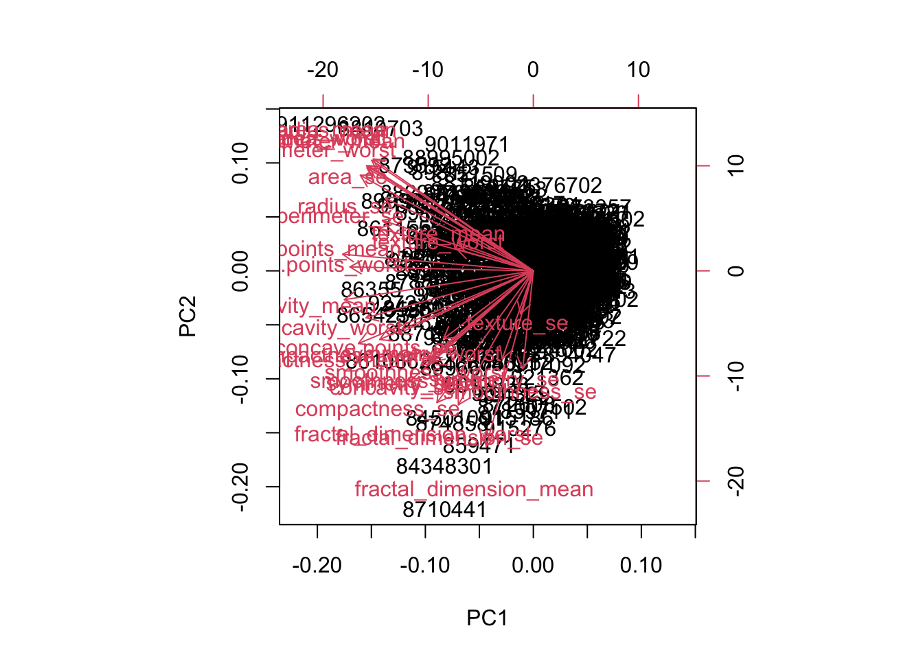
# Scatter plot observations by components 1 and 2
plot(wisc.pr$x[, c(1, 2)], col = (diagnosis + 1),
xlab = "PC1", ylab = "PC2")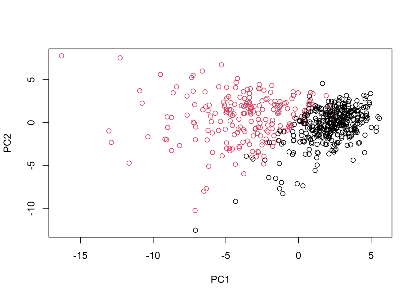
# Repeat for components 1 and 3
plot(wisc.pr$x[, c(1, 3)], col = (diagnosis + 1),
xlab = "PC1", ylab = "PC3")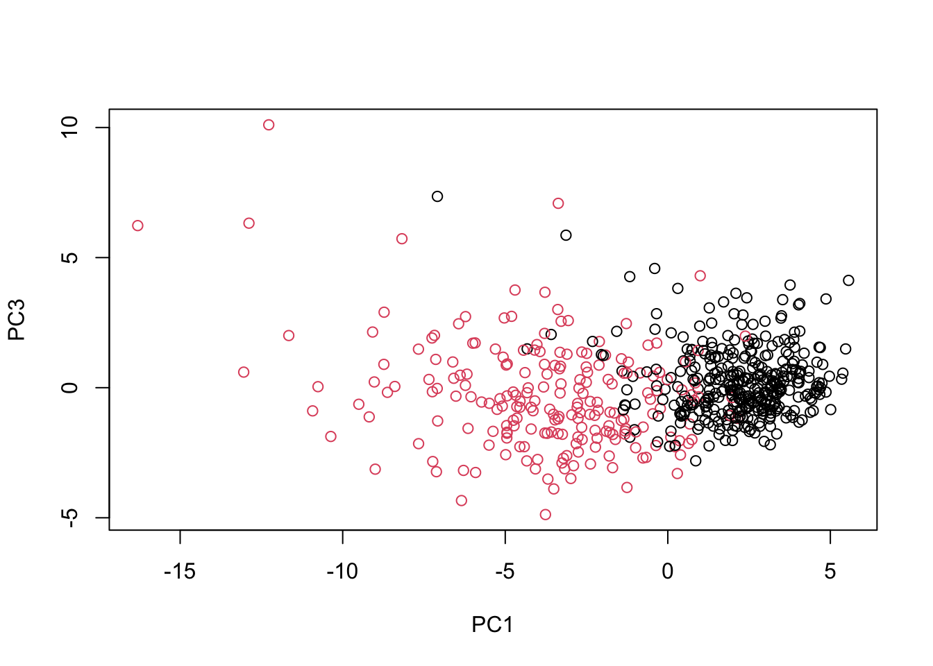
# Do additional data exploration of your choosing below (optional)Excellent work! Because principal component 2 explains more variance in the original data than principal component 3, you can see that the first plot has a cleaner cut separating the two subgroups.
# Set up 1 x 2 plotting grid
par(mfrow = c(1, 2))
# Calculate variability of each component
pr.var <- wisc.pr$sdev^2
# Variance explained by each principal component: pve
pve <- pr.var /sum(pr.var)
# Plot variance explained for each principal component
plot(pve, xlab = "Principal Component",
     ylab = "Proportion of Variance Explained",
     ylim = c(0, 1), type = "b")
# Plot cumulative proportion of variance explained
plot(cumsum(pve), xlab = "Principal Component",
ylab = "Cumulative Proportion of Variance Explained",
ylim = c(0, 1), type = "b")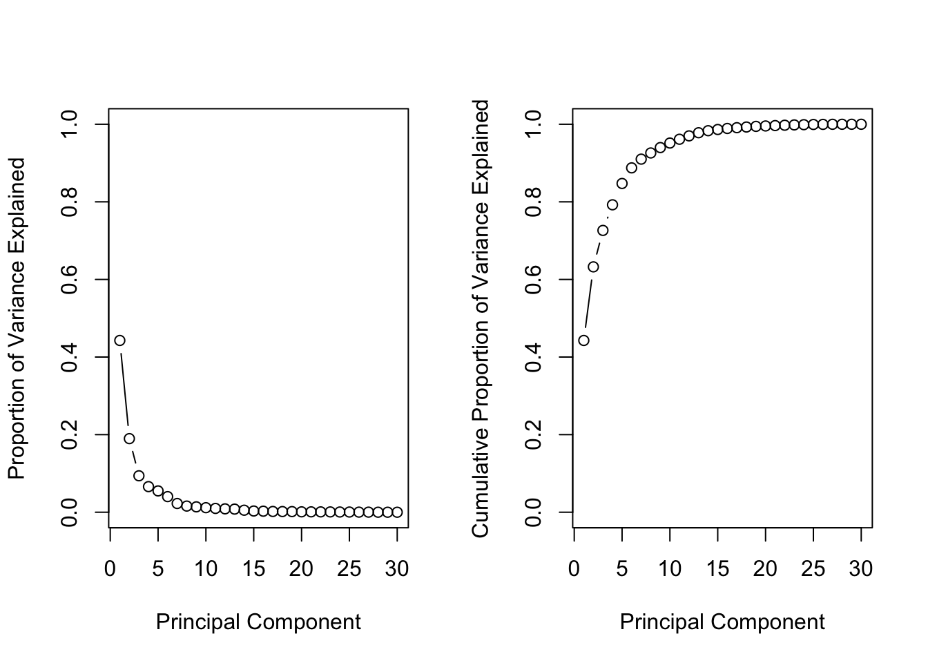
Great work! Before moving on, answer the following question: What is the minimum number of principal components needed to explain 80% of the variance in the data? Write it down as you may need this in the next exercise :)
Hierarchical clustering
# Scale the wisc.data data: data.scaled
data.scaled <- scale(wisc.data)

# Calculate the (Euclidean) distances: data.dist
data.dist <- dist(data.scaled)

# Create a hierarchical clustering model: wisc.hclust
wisc.hclust <- hclust(data.dist, method = "complete")plot(wisc.hclust)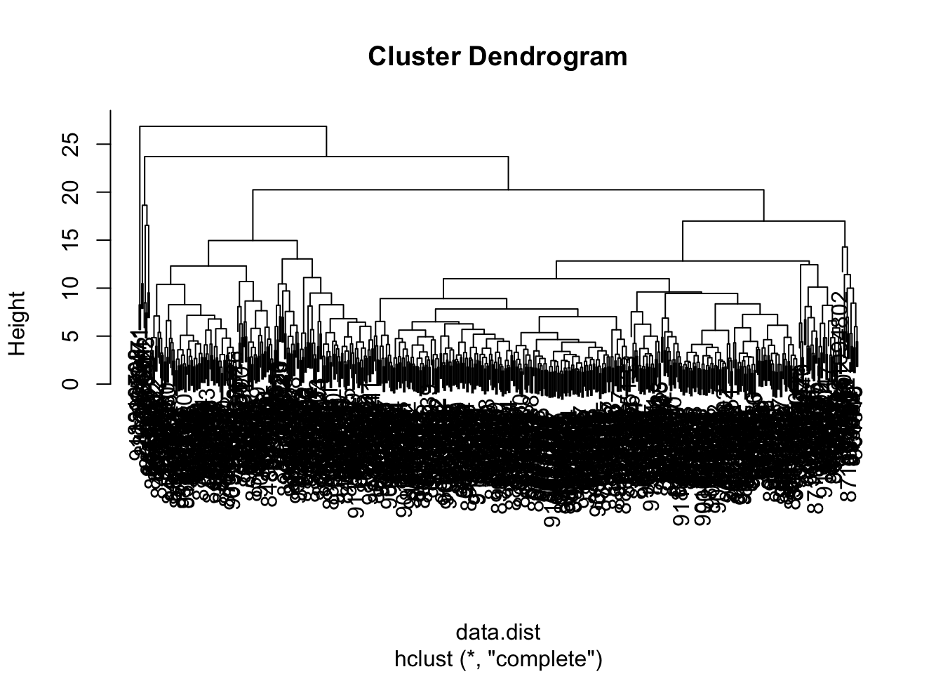
In this exercise, you will compare the outputs from your hierarchical clustering model to the actual diagnoses. Normally when performing unsupervised learning like this, a target variable isn’t available. We do have it with this dataset, however, so it can be used to check the performance of the clustering model.
When performing supervised learning—that is, when you’re trying to predict some target variable of interest and that target variable is available in the original data—using clustering to create new features may or may not improve the performance of the final model. This exercise will help you determine if, in this case, hierarchical clustering provides a promising new feature.
# Cut tree so that it has 4 clusters: wisc.hclust.clusters
wisc.hclust.clusters <- cutree(wisc.hclust, k = 4)

# Compare cluster membership to actual diagnoses
table(wisc.hclust.clusters, diagnosis)
diagnosis
wisc.hclust.clusters 0 1
1 12 165
2 2 5
3 343 40
4 0 2Four clusters were picked after some exploration. Before moving on, you may want to explore how different numbers of clusters affect the ability of the hierarchical clustering to separate the different diagnoses. Great job!
# Create a k-means model on wisc.data: wisc.km
wisc.km <- kmeans(scale(wisc.data), centers = 2, nstart = 20)

# Compare k-means to actual diagnoses
table(wisc.km$cluster, diagnosis)
diagnosis
0 1
1 343 37
2 14 175# Compare k-means to hierarchical clustering
table(wisc.hclust.clusters, wisc.km$cluster)
wisc.hclust.clusters   1   2
                   1  17 160
                   2   0   7
                   3 363  20
                   4   0   2
Nice! Looking at the second table you generated, it looks like clusters 1, 2, and 4 from the hierarchical clustering model can be interpreted as the cluster 1 equivalent from the k-means algorithm, and cluster 3 can be interpreted as the cluster 2 equivalent.
In this final exercise, you will put together several steps you used earlier and, in doing so, you will experience some of the creativity that is typical in unsupervised learning
Recall from earlier exercises that the PCA model required significantly fewer features to describe 80% and 95% of the variability of the data. In addition to normalizing data and potentially avoiding overfitting, PCA also uncorrelates the variables, sometimes improving the performance of other modeling techniques.
Let’s see if PCA improves or degrades the performance of hierarchical clustering.
Using the minimum number of principal components required to describe at least 90% of the variability in the data, create a hierarchical clustering model with complete linkage. Assign the results to wisc.pr.hclust.
# Create a hierarchical clustering model: wisc.pr.hclust
summary(wisc.pr)
Importance of components:
PC1 PC2 PC3 PC4 PC5 PC6 PC7
Standard deviation 3.6444 2.3857 1.67867 1.40735 1.28403 1.09880 0.82172
Proportion of Variance 0.4427 0.1897 0.09393 0.06602 0.05496 0.04025 0.02251
Cumulative Proportion 0.4427 0.6324 0.72636 0.79239 0.84734 0.88759 0.91010
PC8 PC9 PC10 PC11 PC12 PC13 PC14
Standard deviation 0.69037 0.6457 0.59219 0.5421 0.51104 0.49128 0.39624
Proportion of Variance 0.01589 0.0139 0.01169 0.0098 0.00871 0.00805 0.00523
Cumulative Proportion 0.92598 0.9399 0.95157 0.9614 0.97007 0.97812 0.98335
PC15 PC16 PC17 PC18 PC19 PC20 PC21
Standard deviation 0.30681 0.28260 0.24372 0.22939 0.22244 0.17652 0.1731
Proportion of Variance 0.00314 0.00266 0.00198 0.00175 0.00165 0.00104 0.0010
Cumulative Proportion 0.98649 0.98915 0.99113 0.99288 0.99453 0.99557 0.9966
PC22 PC23 PC24 PC25 PC26 PC27 PC28
Standard deviation 0.16565 0.15602 0.1344 0.12442 0.09043 0.08307 0.03987
Proportion of Variance 0.00091 0.00081 0.0006 0.00052 0.00027 0.00023 0.00005
Cumulative Proportion 0.99749 0.99830 0.9989 0.99942 0.99969 0.99992 0.99997
PC29 PC30
Standard deviation 0.02736 0.01153
Proportion of Variance 0.00002 0.00000
Cumulative Proportion 1.00000 1.00000wisc.pr.hclust <- hclust(dist(wisc.pr$x[, 1:7]), method = "complete")
# Cut model into 4 clusters: wisc.pr.hclust.clusters
wisc.pr.hclust.clusters <- cutree(wisc.pr.hclust, k = 4)
# Compare to actual diagnoses
table(diagnosis, wisc.pr.hclust.clusters) wisc.pr.hclust.clusters
diagnosis 1 2 3 4
0 5 350 2 0
1 113 97 0 2# Compare to k-means and hierarchical
table(diagnosis, wisc.hclust.clusters) wisc.hclust.clusters
diagnosis 1 2 3 4
0 12 2 343 0
1 165 5 40 2table(diagnosis, wisc.km$cluster)
diagnosis   1   2
        0 343  14
        1  37 175
Clustering Course
Steps for clustering:
- Preprocessing (making sure ready for analysis, no missing values, features on similar scales, etc)
- Choose similarity metric
- Use a clustering method to group observations based on similarity into clusters
- Analyze output of clusters to see how they provide insight
May neet to iterate 2-4 to see what metrics best add insight on data
Similarity
How similar (or dissimilar) are two observations? Most metrics measure the dissimilarity metric, often referred to as “distance”
Simplest distance is Euclidean distance, the hypoteneuse of a triangle formed by vertical (y) & horizontal distance (x) between them.
in R, dist() function, e.g. dist(x, method = "euclidean").
Can get distance between more than 2 points. Get distance pairwise between points to see which pair has smallest distance.
Ex
two_players <- data.frame(x = c(5, 15),
                          y = c(4, 10))
# output
x y
1 5 4
2 15 10library(tidyverse)── Attaching core tidyverse packages ──────────────────────── tidyverse 2.0.0 ──
✔ dplyr 1.1.4 ✔ readr 2.1.4
✔ forcats 1.0.0 ✔ stringr 1.5.0
✔ ggplot2 3.5.1 ✔ tibble 3.2.1
✔ lubridate 1.9.2 ✔ tidyr 1.3.1
✔ purrr 1.0.2
── Conflicts ────────────────────────────────────────── tidyverse_conflicts() ──
✖ dplyr::filter() masks stats::filter()
✖ dplyr::lag() masks stats::lag()
ℹ Use the conflicted package (<http://conflicted.r-lib.org/>) to force all conflicts to become errors# Plot the positions of the players
ggplot(two_players, aes(x = x, y = y)) +
geom_point() +
# Assuming a 40x60 field
lims(x = c(-30,30), y = c(-20, 20))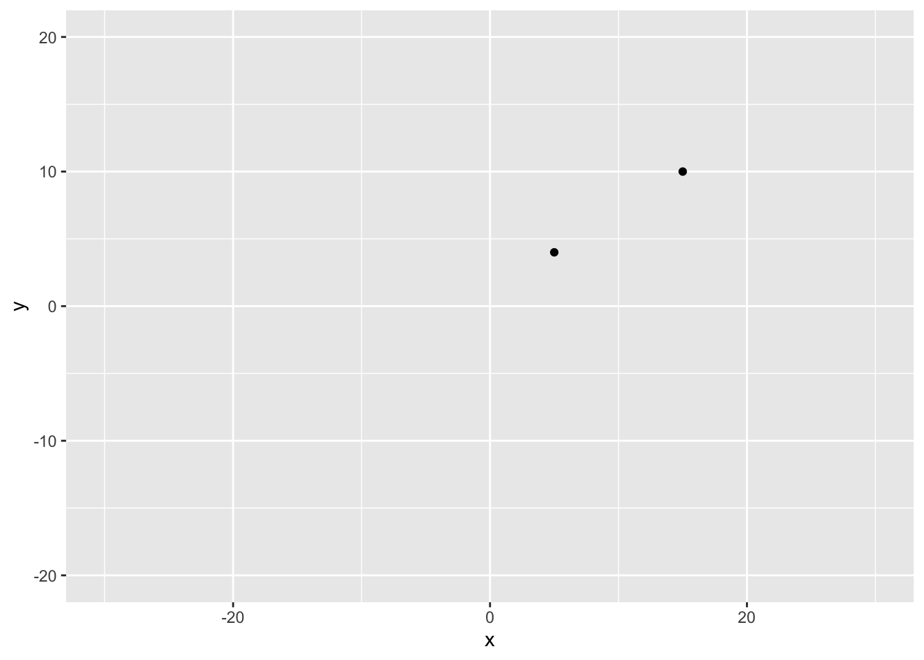
# Split the players data frame into two observations
player1 <- two_players[1, ]
player2 <- two_players[2, ]

# Calculate and print their distance using the Euclidean Distance formula
player_distance <- sqrt( (player1$x - player2$x)^2 + (player1$y - player2$y)^2 )
player_distance
[1] 11.6619three_players <- data.frame(x = c(5, 15, 0),
y = c(4, 10, 30))# Calculate the Distance Between two_players
dist_two_players <- dist(two_players)
dist_two_players
# Calculate the Distance Between three_players
dist_three_players <- dist(three_players)
dist_three_playersImportance of Scale
Features need to be on similar scales. Convert them by standardizing: subtracting mean, dividing by SD.
Ex
# Calculate distance for three_trees
dist_trees <- dist(three_trees)

# Scale three trees & calculate the distance
scaled_three_trees <- scale(three_trees)
dist_scaled_trees <- dist(scaled_three_trees)

# Output the results of both Matrices
print('Without Scaling')
dist_trees

print('With Scaling')
dist_scaled_trees
Notice that before scaling observations 1 & 3 were the closest but after scaling observations 1 & 2 turn out to have the smallest distance.
Measuring Distance for Categorical Data
Consider binary data
Use similarity score called Jaccard Index:
Ratio between intersection of A and B to the union of A and B, i.e. number of times features of both observations are TRUE to the number of times they are ever TRUE.
Ex:
| wine | beer | whiskey | vodka |
|---|---|---|---|
| TRUE | TRUE | FALSE | FALSE |
| FALSE | TRUE | TRUE | TRUE |
Observations 1 and 2 only agree in one category: beer, so only 1 intersection of obs 1 & 2. Number of categories these observations are ever true is 4.
Distance is 1 - similarity, so
To calculate in R, use dist(data, method = "binary")
More than 2 Categories
Need to use dummification to make dummies for each category. Use from the dummies library the dummy.data.frame(data_df) function to preprocess then calculate Jaccard distance.
Example
job_survey
  job_satisfaction is_happy
1               Hi       No
2               Hi       No
3               Hi       No
4               Hi      Yes
5              Mid       No
# Dummify the Survey Data
dummy_survey <- dummy.data.frame(job_survey)
# Calculate the Distance
dist_survey <- dist(dummy_survey, method = "binary")
# Print the Original Data
job_survey
# Print the Distance Matrix
dist_surveyoutput
# Print the Original Data
job_survey
  job_satisfaction is_happy
1               Hi       No
2               Hi       No
3               Hi       No
4               Hi      Yes
5              Mid       No
# Print the Distance Matrix
dist_survey
          1         2         3         4
2 0.0000000
3 0.0000000 0.0000000
4 0.6666667 0.6666667 0.6666667
5 0.6666667 0.6666667 0.6666667 1.0000000
Notice that this distance metric successfully captured that observations 1 and 2 are identical (distance of 0)
We clearly don’t have enough information to make this decision about which player is close to player 1 and player 2, without knowing how we compare one observation to a pair of observations.
The decision required is known as the linkage method and which you will learn about in the next chapter!
Comparing More than 2 Observations - Linkage Methods
Must decide how to measure distance from group of closest observations (a cluster), say points (1,4) to another observation.
One approach is to measure the maximum distance of each observation to the two members of the group (cluster). This is the complete linkage criteria
So point 3 is closer to the cluster.
Hierarchical clustering follows this logic.
The decision of how to select the closest observation to an existing group is called a linkage criteria.
Common linkage criteria:
- complete linkage: maximum distance between two sets
- single linkage: minimum distance between two sets
- average linkage: average distance between two sets
ex
# Extract the pair distances
distance_1_2 <- dist_players[1]
distance_1_3 <- dist_players[2]
distance_2_3 <- dist_players[3]

# Calculate the complete distance between group 1-2 and 3
complete <- max(c(distance_1_2, distance_2_3))
complete

# Calculate the single distance between group 1-2 and 3
single <- min(c(distance_1_2, distance_2_3))
single

# Calculate the average distance between group 1-2 and 3
average <- mean(c(distance_1_2, distance_2_3))
average
output
# Calculate the complete distance between group 1-2 and 3
complete <- max(c(distance_1_2, distance_2_3))
complete
[1] 18.02776
# Calculate the single distance between group 1-2 and 3
single <- min(c(distance_1_2, distance_2_3))
single
[1] 11.6619
# Calculate the average distance between group 1-2 and 3
average <- mean(c(distance_1_2, distance_2_3))
average
[1] 14.84483