Optimization in Python

Mathematical Optimization

Optimization: finding the ideal inputs for a specific problem

e.g. in agriculture, maximize crop yields by analyzing variables like soil condition and weather
e.g. in supply chains, optimal distribution routes by considering distance and traffic

Objective function: describes mathematical relationship between input variables and desired result to be optimized

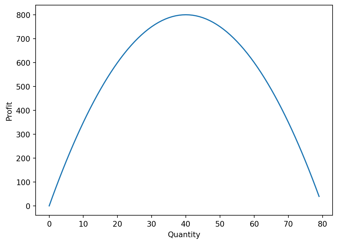
example, profit function depending on output quantity

$P = 40 q - 0.5 q^{2}$

which value of $q$ maximizes $P$ ?

import numpy as np
import matplotlib.pyplot as plt

# create numpy array of quantity values, a range of 80
qs = np.arange(80)

# define objective function
def profit(q):
  return 40 * q - 0.5 * q**2

# plot
plt.plot(qs, profit(qs))
plt.xlabel('Quantity')
plt.ylabel('Profit')
plt.show()

One method: exhaustive search, a “brute force” method: calculate profit for a range of quantities and select the one with the highest profit

# calculate profit for every value in quantities array qs
profits = profit(qs)

# use .max() array method to see which value has profit maximized
max_profit = profits.max()

# find index of the maximum profit in profits array
max_ind = np.argmax(profits) 

q_opt = qs[max_ind] # subset quantity with that index value from qs array

# print a formatted string ("f-string") specified with f before quotes
print(f"The optimum is {q_opt} pieces of furniture, which makes ${max_profit} profit.")

The optimum is 40 pieces of furniture, which makes $800.0 profit.

This method is simple, doesn’t need expensive software, and requires minimal assumptions. But will not scale for complex cases. As complexity increases, brute force becomes rapidly inefficient

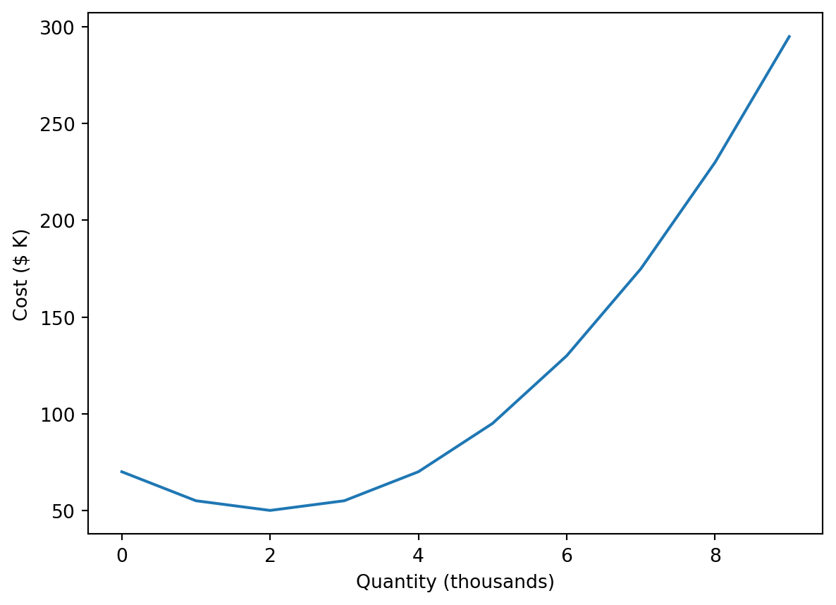
Example

# Create an array of integers from 0 to 10
quantity = np.arange(10)

# Define the cost function
def cost(q): 
  return 50 + 5 * (q - 2) ** 2

# Plot cost versus quantity
plt.plot(quantity, cost(quantity))
plt.xlabel('Quantity (thousands)')
plt.ylabel('Cost ($ K)')
plt.show()

# Calculate the profit for every quantity
profits = profit(quantity)

# Find the maximum profit
max_profit = profits.max()

# Find the optimal quantity
max_profit_ind = np.argmax(profits)
optimal_quantity = quantity[max_profit_ind]

# Print the results
print(f"You need to print {optimal_quantity * 1000} magazines to make the maximum profit of ${max_profit * 1000}.")

You need to print 9000 magazines to make the maximum profit of $319500.0.

You need to print 5000 magazines to make the maximum profit of $11000.

Univariate optimiation

Use calculus, calculate derivative of objective function with sympy package

from sympy import symbols, diff, solve

q = symbols('q') # converts variable name into symbols

P = 40 * q - 0.5 * q**2

# find derivative
dp_dq = diff(P) # differentiate
print(f"The derivative is: {dp_dq}")

The derivative is: 40 - 1.0*q

# find critical point for maximum
q_opt = solve(dp_dq)
print(f"Optimum quantity: {q_opt}")

Optimum quantity: [40.0000000000000]

If second derivative < 0: maximum (concave) If second derivative > 0: minimum (convex)

d2p_dq2 = diff(dp_dq) # take derivative of 1st derivative
#sol = d2p_dq2.subs('q', q_opt)  

# subs() substitutes value into an equation, so once 2nd deriv is found, substitute the optimum quantity and print the result

#print(f"The 2nd derivative is: {sol}")

example

# Convert q into a symbol
q = symbols('q')
c = 2000 - q**2 + 120 * q

# Find the derivative of the objective function
dc_dq = diff(c)
print(f"The derivative is {dc_dq}.")

# Solve the derivative
q_opt = solve(dc_dq)
print(f"Optimum quantity: {q_opt}")

The derivative is 120 - 2*q.
Optimum quantity: [60]

# Find the second derivative
d2c_dq2 = diff(dc_dq)

# Substitute the optimum into the second derivative
#sol = d2c_dq2.subs('q', q_opt)
#print(f"The 2nd derivative at q_opt is: {sol}")

Multivariate Optimization

By calculus, have partial derivatives, how slope changes wtr to each X (holding all others constant)

$F = K^{0.34} L^{0.66}$

In SymPy:

from sympy import symbols, diff, solve

# define variables, K and L (for a production function)
K, L = symbols('K L')
F = K**.34 * L**.66

# partial derivatives
dF_dK = diff(F, K)
dF_dL = diff(F, L)

# solve with a list of the partials and a tuple of symbols they should be solved wrt
crit_points = solve([dF_dK, dF_dL], (K, L))

print(crit_points)

[]

outputs an empty list!

Problem is that our function is increasing indefinitely with each input, has no maxima or minima!

example

# Define symbols K, L
K, L = symbols('K L')

F = -3*K**2 + 100* K - (1/2)*L**2 + 100*L

# Derive the partial derivatives
dF_dK = diff(F, K)
dF_dL = diff(F, L)

# Solve the equations
crit_points = solve([dF_dK, dF_dL], (K, L))
print(crit_points)

{K: 16.6666666666667, L: 100.000000000000}

Unconstrained optimization

SciPy can solve for a minimum in one line of code

from scipy.optimize import minimize_scalar

def objective_function(x):
  return x**2 - 12*x + 4

result = minimize_scalar(objective_function)
print(result)

 message: 
          Optimization terminated successfully;
          The returned value satisfies the termination criteria
          (using xtol = 1.48e-08 )
 success: True
     fun: -32.00000000000001
       x: 6.000000000000001
     nit: 4
    nfev: 9

Printed results attributes, can directly access with result. - fun is the function value at minimum - message provides info on the status of hte process - nfev number of times algorithm evaluated the function - nit number of iterations it took to reach the solution - success boolean on whether optimum was found - x optimal value

result.x

6.000000000000001

Can also find the maximum, but requires a trick

Create a negation of the original function by multiplying it by -1

  -1*(40 * q + 0.5 * q**2)

$- 0.5 q^{2} - 40 q$

def negated_function(q):
  return -40 * q + 0.5 * q**2

result = minimize_scalar(negated_function)
print(f"The maximum is {result.x:.2f} in two decimals")

The maximum is 40.00 in two decimals

Multivariate optimization

for minima

from scipy.optimize import minimize
# minimize requires objects to be in vector form, so only one argument of objective function
# a[0] and a[1] are two variables

def objective_function(a):
  return (a[0] - 2)**2 + (a[1] - 3)**2 + 1.5

# initial guess of correct answer, needed for minimize function
# in array or list
x0 = [1, 2]

result = minimize(objective_function, x0)
print(result)
print(f"minimum is (x, y) = ({result.x[0]:.2f}, {result.x[1]:.2f}) in two decimals.")

  message: Optimization terminated successfully.
  success: True
   status: 0
      fun: 1.5000000000000002
        x: [ 2.000e+00  3.000e+00]
      nit: 2
      jac: [ 0.000e+00  0.000e+00]
 hess_inv: [[ 7.500e-01 -2.500e-01]
            [-2.500e-01  7.500e-01]]
     nfev: 9
     njev: 3
minimum is (x, y) = (2.00, 3.00) in two decimals.

result - hess_inv the inverse of the Hessian, a matrix of all second partial derivatives - jac is Jacobian, the gradient for a scalar function of many variables - status: 0 means process was successful

example

# Define the new objective function
def negated_function(x):
  return -1*(-(x**2) + 3*x - 5)

# Maximize the negated function
result = minimize_scalar(negated_function)

# Print the result
print(f"The maximum is {result.x:.2f} in two decimals")

The maximum is 1.50 in two decimals

def objective_function(a):
  return (a[0] - 2)**2 + (a[1] - 3)**2 + 3 

# Save your initial guess
x0 = [1, 8]

# Calculate and print the minimum
result = minimize(objective_function, x0)
print(f"minimum is (x, y) = ({result.x[0]:.2f}, {result.x[1]:.2f}) in two decimals.")

minimum is (x, y) = (2.00, 3.00) in two decimals.

SciPy’s default solver for unconstrained optimization is Broyden-Fletcher-Goldfarb-Shanno (BFGS), what we’ve been using

A bound-constrained problem: variables limited to a range of values, specified with SciPy’s Bounds class

from scipy.optimize import Bounds

bounds = Bounds(50, 100) # lower and upper bound on range of x

from scipy.optimize import minimize, Bounds

def objective_function(b):
  return (2*b[0] - 1.5*b[1])

bounds = Bounds([5, 10], [25, 30]) # two lists, first the list of lower bounds for b[0] and b[1], second the list of upper bounds

x0 = [10, 5]

result = minimize(objective_function, x0, method = 'L-BFGS-B', bounds = bounds)

print(result.x)

[ 5. 30.]

linear constrained optimization - either the objective function or constraint is linear

here the constraint is linear:

from scipy.optimize import minimize

def objective_function(b):
  return (b[0]) ** 2 + (b[1]) ** 0.5

def constraint_function(x):
  return 2*x[0] + 3*x[1] - 6

# define constraint as a dictionary

# type options are 'eq' and 'ineq'
constraint = {'type': 'ineq',
              'fun': constraint_function}

x0 = [20, 20]

result = minimize(objective_function, x0, constraints = [constraint]) # constraints as a list

print(result)

 message: Optimization terminated successfully
 success: True
  status: 0
     fun: 1.400040565237813
       x: [ 1.203e-01  1.920e+00]
     nit: 8
     jac: [ 2.406e-01  3.609e-01]
    nfev: 25
    njev: 8

example

def objective_function(b):
  return (b[0] - 6)**2 + (b[1] - 8)**2 + 3

# Set the bounds of your problem
bounds = Bounds([2, 2], [100, 100])

x0 = [10, 5]

# Find the minimum
result = minimize(objective_function, x0, bounds = bounds)

print(result.x)

[6.         7.99999999]

def objective_function(b):
  return (b[0] - 5) ** 2 + (b[1] - 3) ** 3

def constraint_function(x):
    return 2*x[0] + 3*x[1] - 6

# Set the constraint variable
constraint = {'type': 'ineq',
              'fun': constraint_function}

x0 = [20, 20]

# Find the minimum
result = minimize(objective_function, x0, constraints = [constraint])

print(result)

 message: Inequality constraints incompatible
 success: False
  status: 4
     fun: -5596424370437617.0
       x: [ 2.665e+05 -1.775e+05]
     nit: 3
     jac: [ 0.000e+00  9.456e+10]
    nfev: 9
    njev: 3

Linear PRogramming

Linear programming: both objective function and constraint function are linear

Objective function: $480 B + 510 C$ Constraints: - machine A: $1.5 B + 1.3 C \leq 4 \times 30$ - machine B: $0.8 B + 2.1 C \leq 3 \times 30$ - Nonnegativity: $B, C \geq 0$

Using PuLP, a library for linear optimization

from pulp import *

model = LpProblem('MaxProfit', LpMaximize) # name of model, and LpMaximize or LpMinimize

# Variables (with nonnegative constraint)
B = LpVariable('B', lowBound = 0)
C = LpVariable('C', lowBound = 0)

# Objective
model += 480*B + 510*C # += adds the objective to the model info
# add constraints with formulas, comma, constraint name
model += 1.5*B + 1.3*C - 120, "M_A"
model += 0.8*B + 2.1*C - 90, "M_B"

print(model)

MaxProfit:
MAXIMIZE
0.8*B + 2.1*C + -90.0
VARIABLES
B Continuous
C Continuous

/Library/Frameworks/Python.framework/Versions/3.10/lib/python3.10/site-packages/pulp/pulp.py:1668: UserWarning: Overwriting previously set objective.
  warnings.warn("Overwriting previously set objective.")

status = model.solve()
print(status)

Welcome to the CBC MILP Solver 
Version: 2.10.3 
Build Date: Dec 15 2019 

command line - /Library/Frameworks/Python.framework/Versions/3.10/lib/python3.10/site-packages/pulp/solverdir/cbc/osx/64/cbc /var/folders/rz/j4p71hkx0pq9h_6fx5z6dq5r0000gn/T/676b5c688a2e47b6802ca5d6591758db-pulp.mps -max -timeMode elapsed -branch -printingOptions all -solution /var/folders/rz/j4p71hkx0pq9h_6fx5z6dq5r0000gn/T/676b5c688a2e47b6802ca5d6591758db-pulp.sol (default strategy 1)
At line 2 NAME          MODEL
At line 3 ROWS
At line 5 COLUMNS
At line 8 RHS
At line 9 BOUNDS
At line 10 ENDATA
Problem MODEL has 0 rows, 2 columns and 0 elements
Coin0008I MODEL read with 0 errors
Option for timeMode changed from cpu to elapsed
Empty problem - 0 rows, 2 columns and 0 elements
Dual infeasible - objective value -0
DualInfeasible objective -0 - 0 iterations time 0.002

Result - Linear relaxation unbounded

Enumerated nodes:           0
Total iterations:           0
Time (CPU seconds):         0.00
Time (Wallclock Seconds):   0.01

Option for printingOptions changed from normal to all
Total time (CPU seconds):       0.00   (Wallclock seconds):       0.02

-2

important is number at bottom: if 1 then we have a solution

print(f"Profit = {value(model.objective):.2f}")
print(f"Tons of bottles = {B.varValue:.2f}, tons of cups = {C.varValue:.2f}")

Profit = -90.00
Tons of bottles = 0.00, tons of cups = 0.00

not working above for some reason…

To handle multiple variables & constraints is to use vectors, matrices, and list comprehensions

variables = LpVariable.dicts("Product", ['B', 'C'], lowBound = 0)

# alternatively

variables = LpVariable.dicts("Product", range(2), 0) # name, dimension (range of 2 for the two elements, or string variables as a list), third is loewr bound

A = LpVariable.matrix('A', (range(2), range(2)), 0) # defines 2x2 matrix and saved as variable A

# use list comprehension and LpSum to define objective function
box_profit = {'B': 480, 'C': 510}

#model += lpSum([box_profit[i] * variables[i] for i in ['B', 'C']])

#model += 1.5*variables['B'] + 1.3*variables['C'] <= 120, "M_A"
#model += 0.8*variables['B'] + 2.1*variables['C'] <= 90, "M_B"

example

PuLP for linear optimization

A farmer faces a diet problem for their cattle. The vet’s recommendation is that each animal is fed at least 7 pounds of a mix of corn and soybean with at least 17% protein and 2% fat. Below are the relevant nutritional elements: Food | type | Cost ($/lb) | Protein (%) | Fat (%) | |—-|——|——–|——–|——-| | corn | 0.11 | 10 | 2.5 | | soybean | 0.28 | 40 | 1 |

You will use this information to minimize costs subject to nutritional constraints.

pulp has been imported for you.

# Define the model
model = LpProblem("MinCost", LpMinimize) 

# Define the variables
C = LpVariable("C", lowBound=0)
S = LpVariable("S", lowBound=0) 

# Add the objective function and constraints
model += 0.11*C + 0.28*S
model += 40*S + 10*C >= 17*(C+S), "M_protein"
model += S + 2.5*C >= 2*(C+S), "M_fat"
model += C + S >= 7, "M_weight"

# Solve the model
model.solve()
print(f"Cost = {value(model.objective):.2f}")
print(f"Pounds of soybean = {S.varValue:.2f}, pounds of corn = {C.varValue:.2f}")

Welcome to the CBC MILP Solver 
Version: 2.10.3 
Build Date: Dec 15 2019 

command line - /Library/Frameworks/Python.framework/Versions/3.10/lib/python3.10/site-packages/pulp/solverdir/cbc/osx/64/cbc /var/folders/rz/j4p71hkx0pq9h_6fx5z6dq5r0000gn/T/7fc4bcb883664e8b8eea310855f6fef3-pulp.mps -timeMode elapsed -branch -printingOptions all -solution /var/folders/rz/j4p71hkx0pq9h_6fx5z6dq5r0000gn/T/7fc4bcb883664e8b8eea310855f6fef3-pulp.sol (default strategy 1)
At line 2 NAME          MODEL
At line 3 ROWS
At line 8 COLUMNS
At line 17 RHS
At line 21 BOUNDS
At line 22 ENDATA
Problem MODEL has 3 rows, 2 columns and 6 elements
Coin0008I MODEL read with 0 errors
Option for timeMode changed from cpu to elapsed
Presolve 3 (0) rows, 2 (0) columns and 6 (0) elements
0  Obj 0 Primal inf 6.9999999 (1)
2  Obj 1.0476667
Optimal - objective value 1.0476667
Optimal objective 1.047666667 - 2 iterations time 0.002
Option for printingOptions changed from normal to all
Total time (CPU seconds):       0.00   (Wallclock seconds):       0.01

Cost = 1.05
Pounds of soybean = 1.63, pounds of corn = 5.37

The farmer wants to replicate the previous optimization function to detail with more complicated meals for other animals on the farm.

The previous code has been provided. Can you adjust the previous code to make it better at handling multiple variables?

Adjust the variable definition to use LpVariable.dicts(), saving them as variables with the name “Food”.

Adjust the objective function to use lpSum().

model = LpProblem("MinCost", LpMinimize) 

# Adjust the variable definition
variables = LpVariable.dicts("Food", ['C', 'S'], lowBound=0)

# Adjust the objective function
cost = {'C': 0.11, 'S': 0.28}
model += lpSum([cost[i] * variables[i] for i in ['C', 'S']]) 

model += 40*variables['S'] + 10*variables['C'] >= 17*(variables['C']+variables['S']), "M_protein"
model += variables['S'] + 2.5*variables['C'] >= 2*(variables['C']+variables['S']), "M_fat"
model += variables['C'] + variables['S'] >= 7, "M_weight"

model.solve()
print(f"Cost = {value(model.objective):.2f}")
print(f"Pounds of soybean = {variables['S'].varValue:.2f}, pounds of corn = {variables['C'].varValue:.2f}")

Welcome to the CBC MILP Solver 
Version: 2.10.3 
Build Date: Dec 15 2019 

command line - /Library/Frameworks/Python.framework/Versions/3.10/lib/python3.10/site-packages/pulp/solverdir/cbc/osx/64/cbc /var/folders/rz/j4p71hkx0pq9h_6fx5z6dq5r0000gn/T/4f7c02d0d2de454a8b50c930a79c659f-pulp.mps -timeMode elapsed -branch -printingOptions all -solution /var/folders/rz/j4p71hkx0pq9h_6fx5z6dq5r0000gn/T/4f7c02d0d2de454a8b50c930a79c659f-pulp.sol (default strategy 1)
At line 2 NAME          MODEL
At line 3 ROWS
At line 8 COLUMNS
At line 17 RHS
At line 21 BOUNDS
At line 22 ENDATA
Problem MODEL has 3 rows, 2 columns and 6 elements
Coin0008I MODEL read with 0 errors
Option for timeMode changed from cpu to elapsed
Presolve 3 (0) rows, 2 (0) columns and 6 (0) elements
0  Obj 0 Primal inf 6.9999999 (1)
2  Obj 1.0476667
Optimal - objective value 1.0476667
Optimal objective 1.047666667 - 2 iterations time 0.002
Option for printingOptions changed from normal to all
Total time (CPU seconds):       0.00   (Wallclock seconds):       0.00

Cost = 1.05
Pounds of soybean = 1.63, pounds of corn = 5.37

Nonlinear constrained optimization

Convex constrained optimization, or mixed integer lienar programming
- convex function is U-shaped
- constraint: limitation on variables
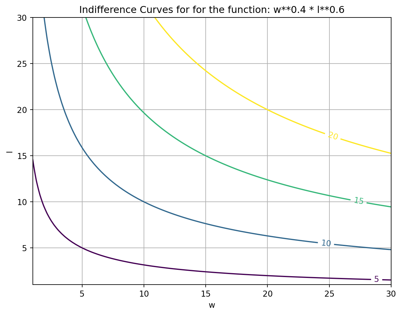
- indifference curve: represents combination of variables
- find point on curve that min/max the objective function
work and leisure

$U (w, l) = w^{0} .4 l^{0} .6$

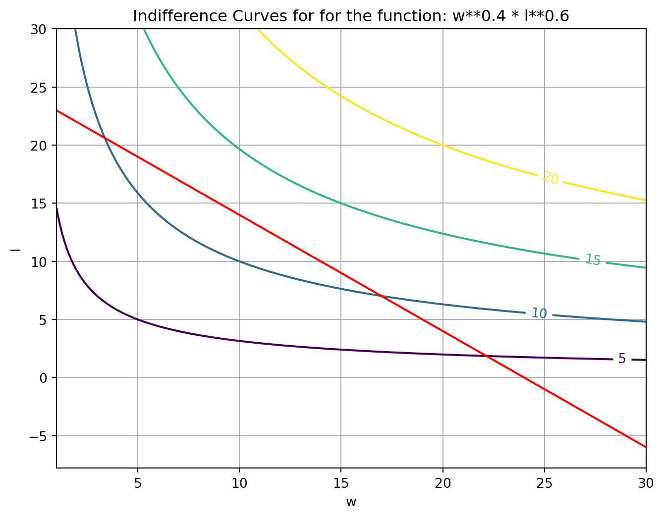
visualize indifference curve by plotting diff values of w and l with numpy and matplotlib

import numpy as np
import matplotlib.pyplot as plt

# define some values for w and l, e.g. 100 values between 1 and 30
w = np.linspace(1, 30, 100)
l = np.linspace(1, 30, 100)
W, L = np.meshgrid(w, l) # meshgrid creates combos of w and l
F = W**0.4 * L**0.6 # objective function

plt.figure(figsize=(8,6))
contours = plt.contour(W, L, F, levels = [5, 10, 15, 20]) # utility levels
plt.clabel(contours)
plt.title("Indifference Curves for for the function: w**0.4 * l**0.6")
plt.xlabel("w")
plt.ylabel("l")
plt.grid(True)
plt.show()

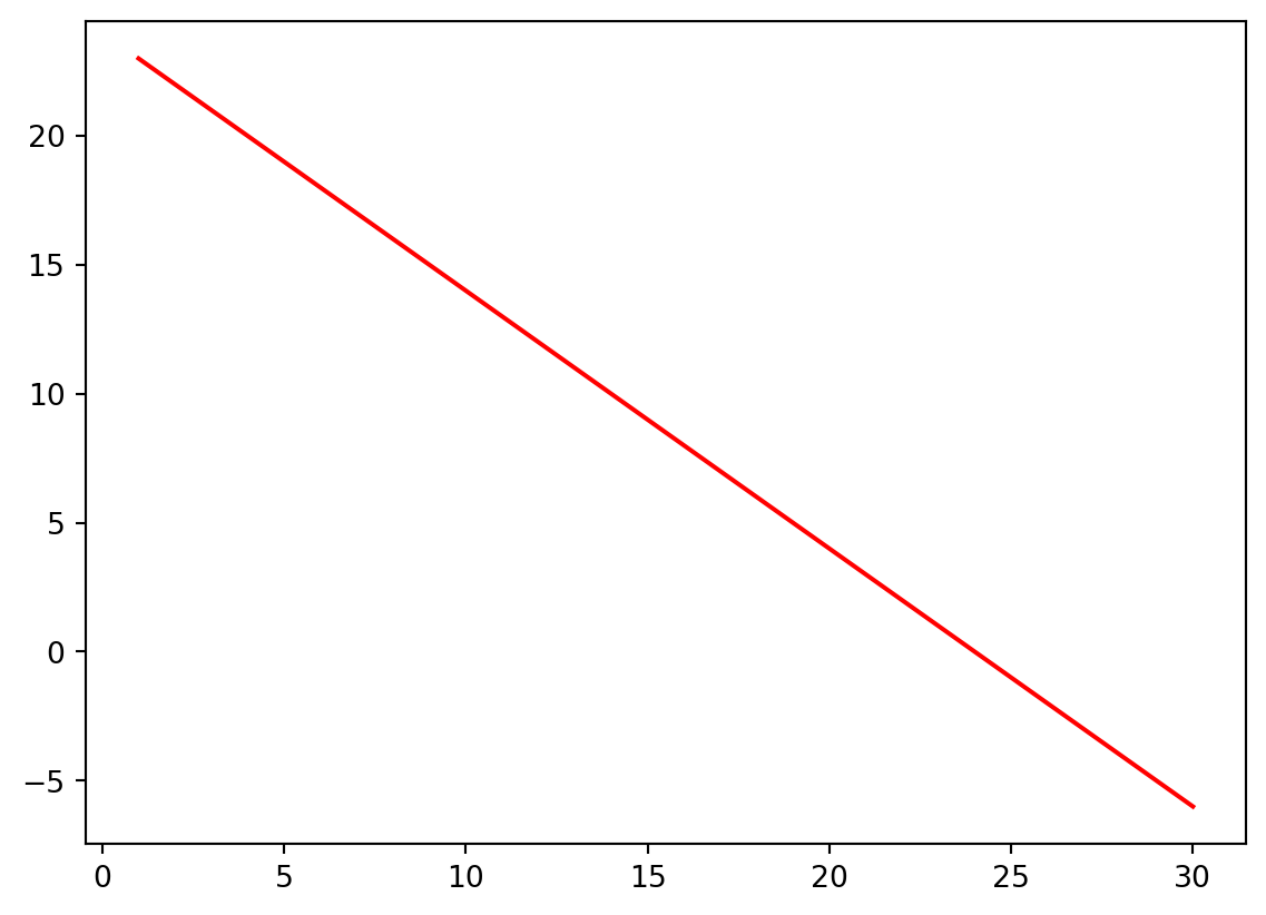
time constrant: 24 hours

$max w, l w^{0} .4 l^{0} .6 s . t . w + l = 24$

Add onstraint to the graph

l = 24 - w
plt.plot(w, l, color = 'red')

import numpy as np
import matplotlib.pyplot as plt

# define some values for w and l, e.g. 100 values between 1 and 30
w = np.linspace(1, 30, 100)
l = np.linspace(1, 30, 100)
W, L = np.meshgrid(w, l) # meshgrid creates combos of w and l
F = W**0.4 * L**0.6 # objective function

plt.figure(figsize=(8,6))
contours = plt.contour(W, L, F, levels = [5, 10, 15, 20]) # utility levels
plt.clabel(contours)
plt.title("Indifference Curves for for the function: w**0.4 * l**0.6")
plt.xlabel("w")
plt.ylabel("l")
plt.grid(True)
l = 24 - w
plt.plot(w, l, color = 'red')

solving with SciPy

def utility_function(vars):
  w, l = vars
  return -(w**0.4 * l**0.6) # negated since we want a maximum

def constraint(vars):
  return 24 - np.sum(vars)

initial_guess = [12, 12]
constraint_definition = {'type': 'eq',
                         'fun': constraint}
result = minimize(utility_function, initial_guess, constraints = constraint_definition)
print(result.x)

[ 9.60001122 14.39998878]

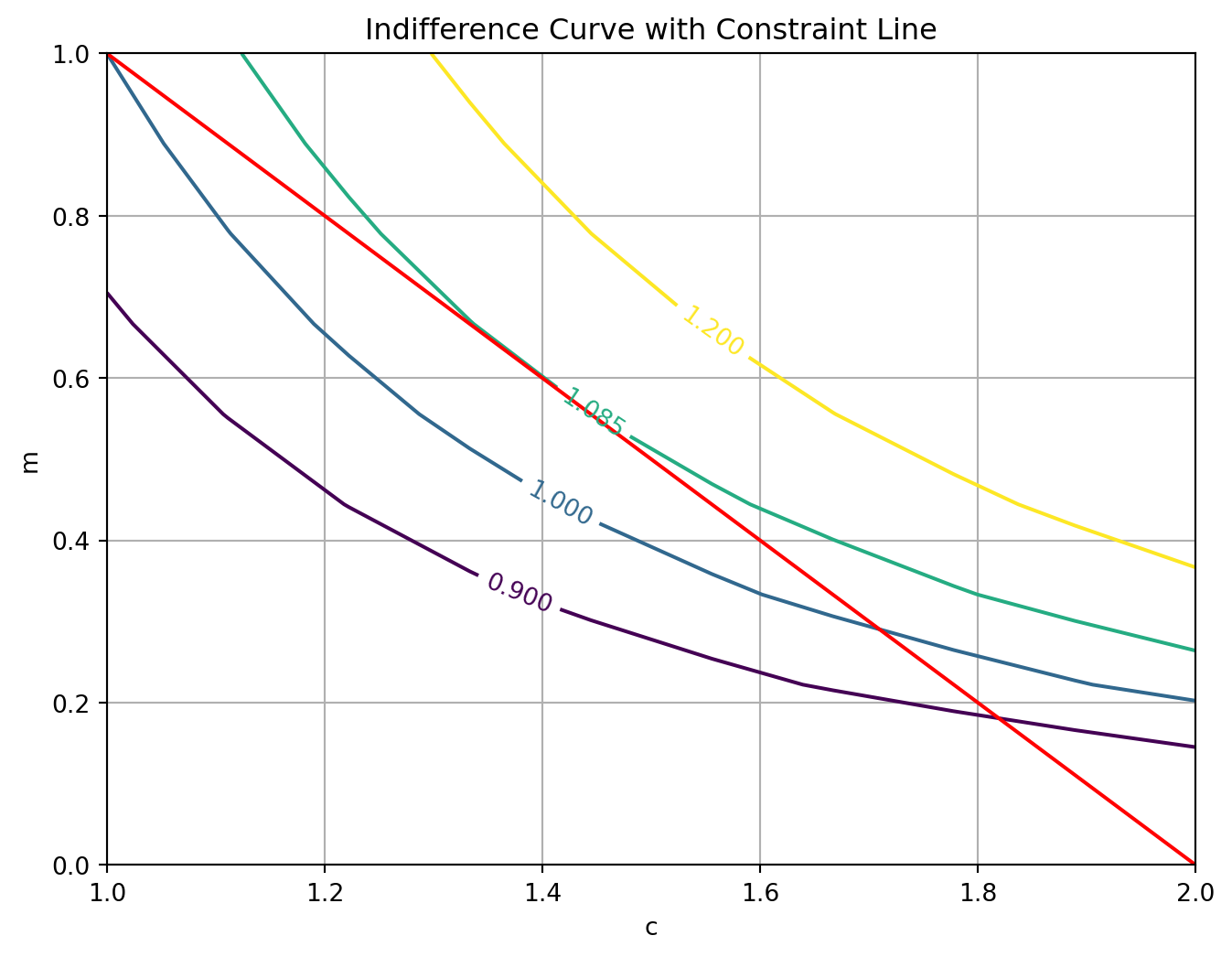
examples

$max c, m c^{0} .7 m^{0} .3 s . t . c + m = 2$

import numpy as np
import matplotlib.pyplot as plt

c = np.linspace(1, 2, 10)  
# Define the constraint and generate combinations
m = 2 - c
C, M = np.meshgrid(c, m)
# Define the utility function
F = C**0.7 * M**0.3

plt.figure(figsize=(8, 6))
# Plot the controls and constraints
contours = plt.contour(C, M, F, levels=[0.9, 1.00, 1.085, 1.2])
plt.clabel(contours)
plt.plot(c, m, color='red')
plt.title('Indifference Curve with Constraint Line')
plt.xlabel('c')
plt.ylabel('m')
plt.grid(True)
plt.show()

# Define the utility function
def utility_function(vars):
    c, m = vars
    return -(c**0.7 * m**0.3)

# Define the constraint function
def constraint(vars):
    return 2 - np.sum(vars)

initial_guess = [12, 12]  

# Set up the constraint
constraint_definition = {'type': 'eq',
                         'fun': constraint}

# Perform optimization
result = minimize(utility_function, initial_guess, constraints = constraint_definition)
c,m = result.x

print("Optimal study hours for classical music:", round(c, 2))
print("Optimal study hours for modern music:", round(m, 2))

Optimal study hours for classical music: 1.4
Optimal study hours for modern music: 0.6

Convex-constrained optimization with inequality constraints

Corner solution vs. interior solution
- Corner solution: two linear contraints -> intersection is a corner solution
- Interior solution: not an intersection or corner

Consider manufacturer with capacity constraints, producing in two factories $A$ and $B$ : - Quantities $q_{A}$ , $q_{B}$ - Capacities: $q_{A} \leq 90$ , $q_{B} \leq 90$ - Cost: $C_{A} (q) = 3 q$ , $C_{B} (q) = 3.5 q$ - Demand: $P = 120 - Q$ - Contract: $Q \geq 92$ - Objective: $m a x Π (q_{A}, q_{B})$

$$ $\begin{aligned} Π & = R - C \\ Π & = P Q \\ Π & = (120 - Q) Q - 3 q_{A} + 3.5 q_{B} \end{aligned}$ $$

Bounds: $0 \leq q_{A}, q_{B} \leq 90$ Constraints: $92 \leq q_{A} + q_{B}$

from scipy.optimize import minimize, \
  Bounds, LinearConstraint

def R(q):
  return (120 - (q[0]  + q[1]
  )) * (q[0] + q[1])

def C(q): return 3*q[0] + 3.5*q[1]

def profit(q): return R(q) - C(q)

bounds = Bounds([0, 0], [90, 90])

constraints = LinearConstraint([1, 1], lb=92) 
  # first arg: coefs from each constraint function, each output from qA and qB counts 1 towards Q
  # second arg: lower bound

result = minimize(lambda q: -profit(q), # negate the profit function to get maximum, using a lambda function here
                  [50, 50], # initial guess
                  bounds = bounds,
                  constraints = constraints) 

print(result.message)
print(f'The optimal number of cars produced in plant A is: {result.x[0]:.2f}')
print(f'The optimal number of cars produced in plant B is: {result.x[1]:.2f}')
print(f'The firm made: ${-result.fun:.2f}') # take negative to cancel out original negation

Optimization terminated successfully
The optimal number of cars produced in plant A is: 90.00
The optimal number of cars produced in plant B is: 2.00
The firm made: $2299.00

For nonlinear constraints (example)

from scipy.optimize import NonlinearConstraint
import numpy as np

constraints = NonlinearConstraint(lambda q: q[0] + q[1], lb = 92, ub = np.Inf)

# result is the same

example

Linear constrained biscuits

Congratulations! Your biscuit business has expanded. You now have two bakeries, $A$ and $B$ to help you deliver your biscuits nationwide.

Your bakeries can each make 100 biscuits a day and the cost of making a biscuit in bakery $A$ is 1.5 times the quantity $q$ while in bakery $B$ it is $1.75 q$ .

Price is defined by $150 - q$

Your business is booming and you already have 140 biscuit pre-orders for the day. You want to maximize your profit for the day. How many biscuits should you make in each bakery?

minimize, Bounds, and LinearConstraint have been loaded for you and the revenue function R is already defined.

def R(q):
    return (150 - q[0] - q[1]) * (q[0] + q[1])

# Define the cost function
def C(q): 
  return 1.5*q[0] + 1.75*q[1]

# Define the profit function
def profit(q): 
  return R(q) - C(q)

# Define the bounds and constraints
bounds = Bounds([0,0], [100,100]) 
constraints = LinearConstraint([1, 1], lb=140) 

# Perform optimization
result = minimize(lambda q: -profit(q),                 
                  [50, 50],              
                  bounds=bounds,
                  constraints=constraints)

print(result.message)
print(f'The optimal number of biscuits to bake in bakery A is: {result.x[0]:.2f}')
print(f'The optimal number of biscuits to bake in bakery A is: {result.x[1]:.2f}')
print(f'The bakery company made: ${-result.fun:.2f}')

Optimization terminated successfully
The optimal number of biscuits to bake in bakery A is: 100.00
The optimal number of biscuits to bake in bakery A is: 40.00
The bakery company made: $1180.00

Nonlinear constrained biscuits

That was some excellent baking!

Now can you solve the same problem again using NonlinearConstraint?

Recall the constraint for the bakeries is they need to fulfill a minimum of 140 pre-orders and each factory can make 100 biscuits daily.

minimize, Bounds, and NonlinearConstraint have been loaded for you as well as the revenue function R, cost function C, and profit function profit.

from scipy.optimize import NonlinearConstraint

# Redefine the problem with NonlinearConstraint
constraints = NonlinearConstraint(lambda q: q[0] + q[1], lb = 140, ub = np.Inf)

# Perform optimization
result = minimize(lambda q: -profit(q), 
                  [50, 50], 
                  bounds=Bounds([0,0], [100,100]),
                  constraints=constraints)

print(result.message)
print(f'The optimal number of biscuits to bake in bakery A is: {result.x[0]:.2f}')
print(f'The optimal number of biscuits to bake in bakery A is: {result.x[1]:.2f}')
print(f'The bakery company made: ${-result.fun:.2f}')

Optimization terminated successfully
The optimal number of biscuits to bake in bakery A is: 100.00
The optimal number of biscuits to bake in bakery A is: 40.00
The bakery company made: $1180.00

Mixed Integer Linear Programming (MILP)

MILP used when constraint variables are integers or discrete variables

Global Optimization

When there are many good options available - multiple local maxima - common problem is getting stuck in a local optimum

Consider a function with two maxima, at q = 5 and q = 18, and a minimum at q = 10

from scipy.optimize import minimize_scalar, minimize

def profit(q):
  return -q**4 / 4 + 11 * q**3 - 160 * q**2 + 900 * q

result_min_scalar = minimize_scalar(lambda q: -profit(q))

print(f"{result_min_scalar.message}")
print(f"The maximum according to minimize scalar is {-result_min_scalar.fun:.2f} \
  and achieved at {result_min_scalar.x:.2f}\n")


Optimization terminated successfully;
The returned value satisfies the termination criteria
(using xtol = 1.48e-08 )
The maximum according to minimize scalar is 1718.75   and achieved at 5.00

optimum at 5, trapped in a local maximum

x0 = 9

result = minimize(lambda q: -profit(q), x0, bounds = [(0, 20)])
print(f"{result.message}")
print(f"The maximum according to minimize (x0={x0} is {-result.fun:.2f} at {result.x[0]:.2f}\n")

CONVERGENCE: NORM_OF_PROJECTED_GRADIENT_<=_PGTOL
The maximum according to minimize (x0=9 is 1718.75 at 5.00

Provided an initial guess of 9, algorithm will find the smallest of the two local maxima

Worse, if we provide a guess close to the local minima, will be trapped there:

x0 = 10 + 1e-8

result = minimize(lambda q: -profit(q), x0, bounds = [(0, 20)])
print(f"{result.message}")
print(f"The maximum according to minimize (x0={x0} is {-result.fun:.2f} at {result.x[0]:.2f}\n")

CONVERGENCE: REL_REDUCTION_OF_F_<=_FACTR*EPSMCH
The maximum according to minimize (x0=10.00000001 is 1500.00 at 10.00

Use basinhopping to find global maximum

from scipy.optimize import basinhopping

x0 = 0
result = basinhopping(lambda q: -profit(q), x0, niter = 10000) # 10000 iterations

# more iterations is a more thorough but slower search

print(f"{result.message}")
print(f"The maximum according to basinhopping (x0={x0}, niter = 10000 \
   is {-result.fun:.2f} at {result.x[0]:.2f}\n")

['requested number of basinhopping iterations completed successfully']
The maximum according to basinhopping (x0=0, niter = 10000    is 2268.00 at 18.00

basinhopping takes optional args: - kwargs (keyword arguments)

from scipy.optimize import basinhopping, NonlinearConstraint

x0 = 0
kwargs = {"constraints": NonlinearConstraint(lambda x: x, lb=0, ub=30)}

result = basinhopping(lambda q: -profit(q), x0, minimizer_kwargs= kwargs) # 10000 iterations
print(f"The maximum according to basinhopping (x0={x0} is at {result.x[0]:.2f}\n")

The maximum according to basinhopping (x0=0 is at 18.00

good rule is to always provide constraints and bounds if they are known, speeds up finding optimum

adding a callback helps us monitor the process

from scipy.optimize import basinhopping, NonlinearConstraint

x0 = 0
kwargs = {"constraints": NonlinearConstraint(lambda x: x, lb=0, ub=30)}

# create list called maxima
maxima = []

def callback(x, f, accept): 
  # x is current minimum, f is value of objective at x, accept is Boolean = True if basinhopping deems x as local optimum
  if accept:
    maxima.append(*x)

# when basinhopping examines a point it calls callback, which appends that point in the list of maxima

result = basinhopping(lambda q: -profit(q),
                      x0,
                      callback = callback,
                      minimizer_kwargs = kwargs,
                      niter = 5)

print(f"{result.message}")
print(f"The maximum according to basinhopping (x0={x0} is at {result.x[0]:.2f}\n")
print(f"(Local) maxima found by basinhopping are: {[round(x, 2) for x in maxima]}")

['requested number of basinhopping iterations completed successfully']
The maximum according to basinhopping (x0=0 is at 5.00

(Local) maxima found by basinhopping are: [5.0, 5.0, 5.0, 5.0, 5.0, 5.0]

Note that this result is stochastic/random, if we want replicability, set seed.

I didn’t get both maxima in my runs, but the video did.

example

def profit(q): 
    return -q**4 / 4 + 11 * q**3 - 160 * q**2 + 900 * q
  
x0 = 0

# Define the keyword arguments for bounds
kwargs = {"bounds": [(0, 30)]} 

# Run basinhopping to find the optimal quantity
result = basinhopping(lambda q: -profit(q), x0, minimizer_kwargs=kwargs)

print(f"{result.message}")
print(f"The maximum according to basinhopping(x0={x0}) is at {result.x[0]:.2f}\n")

['requested number of basinhopping iterations completed successfully']
The maximum according to basinhopping(x0=0) is at 18.00

opt_values = []

def callback(x, f, accept):
# Check if the candidate is an optimum  
    if accept:
# Append the value of the minimized objective to list opt_values      
        opt_values.append(f)

# Run basinhopping to find top two maxima  
result = basinhopping(lambda q: -profit(q), x0, callback=callback, minimizer_kwargs=kwargs, niter=5, seed=3) 
top2 = sorted(list(set([round(f, 2) for f in opt_values])), reverse=True)[:2]
top2 = [-f for f in top2]

print(f"{result.message}\nThe highest two values are {top2}")

['requested number of basinhopping iterations completed successfully']
The highest two values are [2268.0]

Sensitivity Analysis in PUlP

sensitivity analysis changes one parameter to see changes in outcome
- in linear programming, how much the objective changes at the optimum
- three approaches:
  1. change a coefficient in the objective
  2. change a coefficient in a constraint
  3. change the constant in a constraint

Definitions - satisfied constraint @ optimum is active or binding if it holds with equality - if it holds with strict inequality, it is non-active, non-binding, or slack (adj) - slack (noun) amount added to the left of the constraint to make it binding - binding constraints have 0 slack - shadow price: marginal increase in objective with respect to right of the constraint

consider a cost-minimizing diet problem

Food	Cost ($/lb)	Protein (%)	Fat (%)
corn	0.11	10	2.5
soybean	0.28	40	1

Farmer wishes to feed pigs at minimum cost

Recommended diet contains at least 17% protein, 2% fat, 7 lb of food
Objective: $0.11 C + 0.28 S$
Constraints:
- Protein: $10 C + 40 S \leq 17 (C + S)$
- Fat: $2.5 C + S \leq 2 (C + S)$
- Weight: $C + S > 7$
- dont need to rewrite all this for PulP which is nice

from pulp import *

model = LpProblem('diet', LpMinimize)

C = LpVariable('C', lowBound = 0)
S = LpVariable('S', lowBound = 0)

model += 0.11*C + 0.28*S

model += 10*C + 40*S >= 17 * (C+S), 'Protein'
model += 2.5*C + S >= 2 * (C+S), 'Fat'
model += C + S >= 7, 'Weight'

model.solve()

Welcome to the CBC MILP Solver 
Version: 2.10.3 
Build Date: Dec 15 2019 

command line - /Library/Frameworks/Python.framework/Versions/3.10/lib/python3.10/site-packages/pulp/solverdir/cbc/osx/64/cbc /var/folders/rz/j4p71hkx0pq9h_6fx5z6dq5r0000gn/T/5fd440a719644f0b9148e13c7edab756-pulp.mps -timeMode elapsed -branch -printingOptions all -solution /var/folders/rz/j4p71hkx0pq9h_6fx5z6dq5r0000gn/T/5fd440a719644f0b9148e13c7edab756-pulp.sol (default strategy 1)
At line 2 NAME          MODEL
At line 3 ROWS
At line 8 COLUMNS
At line 17 RHS
At line 21 BOUNDS
At line 22 ENDATA
Problem MODEL has 3 rows, 2 columns and 6 elements
Coin0008I MODEL read with 0 errors
Option for timeMode changed from cpu to elapsed
Presolve 3 (0) rows, 2 (0) columns and 6 (0) elements
0  Obj 0 Primal inf 6.9999999 (1)
2  Obj 1.0476667
Optimal - objective value 1.0476667
Optimal objective 1.047666667 - 2 iterations time 0.002
Option for printingOptions changed from normal to all
Total time (CPU seconds):       0.00   (Wallclock seconds):       0.02

print(f"Status: {LpStatus[model.status]}\n")

Status: Optimal

for name, c in model.constraints.items():
  print(f"{name}: slack = {c.slack:.2f}, shadow price = {c.pi:.2f}")

Protein: slack = -0.00, shadow price = 0.01
Fat: slack = -1.05, shadow price = 0.00
Weight: slack = -0.00, shadow price = 0.15

model.constraints contains ordered dict where key is the name of the constraint and value the constraint along wiht useful info

For protein, when slack = 0, shadow price is positive. When we relax constraint, objective should incraese On other hand, when slack is nonzero, as for fat. Shifting constraint does not affect its slackness, hence the solution and objective remain unaffected, making the shadow price is 0

example

A firm is employing two machines and to put grapefruit juice () and orange juice (

) in bottles. Its goal is to maximize profit subject to the constraints

M1: and M2:

The constraints reflect the productivity and availability of machines. For example, M1 is available for 40 hours per week and needs 6 hours to bottle 1 ton of grapefruit juice and 5.5 hours for a ton of orange juice.

There is an additional supply constraint where the firm only receives a maximum of 6 tons of grapefruit a week, and 12 tons of oranges. These are the upper bounds.

pulp has been imported for you and model has been defined as well as the variables g and o for grapefruit and orange juice.

#print(LpStatus[model.status])
##print(f'The optimal amount of {g.name} embottled is: {g.varValue:.2f} tons')
# print(f'The optimal amount of {o.name} embottled is: {o.varValue:.2f} tons')

#for name, c in model.constraints.items():
    # Check if shadow value is positive 
#    if c.pi > 0:
    # Enter the variable that measures marginal increase in objective when constraint is relaxed
#        print(f"Increasing the capacity of {name} by one unit would increase profit by {c.pi} units.")
#    else:
    # Enter the variable that measures how tight the constraint is
#        print(f"{name} has {c.slack} units of unused capacity.")