Time Series Analysis in R

Time Series in R

R has dedicated classes for time series objects
- ts in BaseR
- zoo from zoo package

AirPassengers

each obs has 2 parts: point in time and value
ggplot2 packages has dedicated autoplot() function for time series objects

library(tidyverse)

── Attaching core tidyverse packages ──────────────────────── tidyverse 2.0.0 ──
✔ dplyr     1.1.4     ✔ readr     2.1.5
✔ forcats   1.0.0     ✔ stringr   1.5.1
✔ ggplot2   3.5.1     ✔ tibble    3.2.1
✔ lubridate 1.9.3     ✔ tidyr     1.3.1
✔ purrr     1.0.2     
── Conflicts ────────────────────────────────────────── tidyverse_conflicts() ──
✖ dplyr::filter() masks stats::filter()
✖ dplyr::lag()    masks stats::lag()
ℹ Use the conflicted package (<http://conflicted.r-lib.org/>) to force all conflicts to become errors

#autoplot(maunaloa)

# Determine the summary statistics of maunaloa
maunaloa %>% summary()

 Index            .

Min. :1974 Min. :326.7
1st Qu.:1986 1st Qu.:347.6
Median :1998 Median :366.1
Mean :1998 Mean :369.2
3rd Qu.:2010 3rd Qu.:389.6
Max. :2022 Max. :421.6

data classes representing temporal/time-based data

numeric: integers or floating-point doubles
- dates stored as numerics represent integer number of days since 1970-01-01 (start of Unix epoch)
character: strings of text
- imported data often represents dates in R as char
- often "2020-08-23", but don’t always conform to this standard
Date represents the day of the year (note the cape)
- printing out looks identical to character "2020-08-23"
- allows us to do math with dates:

start_date <- as.Date("2020-08-23")
end_date <- as.Date("2020-08-30")

end_date - start_date

POSIXct represents date and time (and time zone)
- ct stands for calendar time
- POSIX is a standard for date and time representation
- POSIXct is the number of seconds since 1970-01-01
- POSIXlt is a list of date and time components
- POSIXt is the superclass of POSIXct and POSIXlt
- can also perform math with POSIXct objects
lubridate::as_date() converts a character or numeric date to the Date class
- similar to Base R’s as.Date() but with improvements
  - better performance with time zones
  - warnings for invalid formats
  - easier conversions from numeric

my_date <- as_date("2022-01-20")
my_date

[1] "2022-01-20"

class(my_date)

[1] "Date"

Formatting dates

Order of time elements - In US: mm/dd/yyyy - ISO 8601: yyyy-mm-dd

lubridate::parse_date_time() takes an input character or Date vector and returns a POSIXct vector

earthday <- "April 12, 2024"

parse_date_time(earthday, 
                orders = "%B %d, $Y") # conversion specifications

[1] "2024-04-12 UTC"

Common conversion specifications:

help(strptime) for more details

Time Element	Conversion Spec.
Year (`YYYY`)	`%Y`
Year (`yy`)	`%y`
Day (`dd`)	`%d`
Month (`mm`)	`%m`
Month (`August`)	`%B`
Month (`Aug`)	`%b`

lubridate::ymd() and lubridate::dmy() are shortcuts for parse_date_time() with specific orders

example

# Print the dates_order object
dates_order

[1] “2019-01-01” “2019-01-02” “01/03/2019” “2019-01-04” “2019-01-05” [6] “2019-01-06” “01/07/2019” “2019-01-08” “2019-01-09” “2019-01-10”

# Enter all the date formats from dates_order
parse_date_time(dates_order,
                orders = c("%Y-%m-%d", "%m/%d/%Y"))

[1] “2019-01-01 UTC” “2019-01-02 UTC” “2019-01-03 UTC” “2019-01-04 UTC” [5] “2019-01-05 UTC” “2019-01-06 UTC” “2019-01-07 UTC” “2019-01-08 UTC” [9] “2019-01-09 UTC” “2019-01-10 UTC”

Time Series Attributes

temporal attributes
- start point

start(AirPassengers)  # year 1949 month 1

[1] 1949    1

- might have a fractional date, e.g. 1998.646, a "decimal date" can convert into POSIXct with
- decimal dates might be useful for ensuring time series have evenly-spaced intervals

lubridate::date_decimal(1998.646)

[1] "1998-08-24 18:57:35 UTC"

end point

end(AirPassengers)  # year 1960 month 12

[1] 1960   12

frequency

frequency(AirPassengers)  # 12

[1] 12

Regular vs. irregular time series
- Regular: evenly-spaced intervals
  - No missing values (no missing dates)
  - Uses decimal date for ‘irregular’ intervals (e.g. if data is only on weekdays)
  - Base R
- Irregular: spacing is irregular
  - weekdays, random days
  - missing obs
  - decimal date/POSIXct date
  - zoo package

examples

# Save the start point of maunaloa: maunaloa_start
maunaloa_start <- start(maunaloa)

# Assign the formatted date to start_iso
start_iso <- date_decimal(maunaloa_start)

# Convert to Date class
as_date(start_iso)

# Assign the start point to card_start
card_start <- start(card_prices)

# Assign the end point to card_end
card_end <- end(card_prices)

# Subtract the start point from the end point
card_end - card_start

Time difference of 729 days

Time Series Objects with the `zoo` package

zoo class of objects
functions for manipulating & visualizing time series
vs. baseR’s ts, zoo class objects can be regular or irregular intervals, converted to data.frames

sample_values <- round(rnorm(10, mean = 100, sd = 15),2)
sample_dates <- as.Date("2020-01-01") + 0:9

library(zoo)


Attaching package: 'zoo'

The following objects are masked from 'package:base':

    as.Date, as.Date.numeric

# create a zoo object
my_zoo <- zoo(x = sample_values, # values
              order.by = sample_dates) # index

my_zoo

2020-01-01 2020-01-02 2020-01-03 2020-01-04 2020-01-05 2020-01-06 2020-01-07 
    139.40      95.41      75.13     114.12      89.58     110.95     115.85 
2020-01-08 2020-01-09 2020-01-10 
     88.03      80.98      91.32

older datasets in R are often ts, can convert to zoo

class(AirPassengers)

[1] "ts"

AP_zoo <- as.zoo(AirPassengers)

class(AP_zoo)

[1] "zooreg" "zoo"

# methods are different
print(AirPassengers)

     Jan Feb Mar Apr May Jun Jul Aug Sep Oct Nov Dec
1949 112 118 132 129 121 135 148 148 136 119 104 118
1950 115 126 141 135 125 149 170 170 158 133 114 140
1951 145 150 178 163 172 178 199 199 184 162 146 166
1952 171 180 193 181 183 218 230 242 209 191 172 194
1953 196 196 236 235 229 243 264 272 237 211 180 201
1954 204 188 235 227 234 264 302 293 259 229 203 229
1955 242 233 267 269 270 315 364 347 312 274 237 278
1956 284 277 317 313 318 374 413 405 355 306 271 306
1957 315 301 356 348 355 422 465 467 404 347 305 336
1958 340 318 362 348 363 435 491 505 404 359 310 337
1959 360 342 406 396 420 472 548 559 463 407 362 405
1960 417 391 419 461 472 535 622 606 508 461 390 432

print(AP_zoo)

Jan 1949 Feb 1949 Mar 1949 Apr 1949 May 1949 Jun 1949 Jul 1949 Aug 1949 
     112      118      132      129      121      135      148      148 
Sep 1949 Oct 1949 Nov 1949 Dec 1949 Jan 1950 Feb 1950 Mar 1950 Apr 1950 
     136      119      104      118      115      126      141      135 
May 1950 Jun 1950 Jul 1950 Aug 1950 Sep 1950 Oct 1950 Nov 1950 Dec 1950 
     125      149      170      170      158      133      114      140 
Jan 1951 Feb 1951 Mar 1951 Apr 1951 May 1951 Jun 1951 Jul 1951 Aug 1951 
     145      150      178      163      172      178      199      199 
Sep 1951 Oct 1951 Nov 1951 Dec 1951 Jan 1952 Feb 1952 Mar 1952 Apr 1952 
     184      162      146      166      171      180      193      181 
May 1952 Jun 1952 Jul 1952 Aug 1952 Sep 1952 Oct 1952 Nov 1952 Dec 1952 
     183      218      230      242      209      191      172      194 
Jan 1953 Feb 1953 Mar 1953 Apr 1953 May 1953 Jun 1953 Jul 1953 Aug 1953 
     196      196      236      235      229      243      264      272 
Sep 1953 Oct 1953 Nov 1953 Dec 1953 Jan 1954 Feb 1954 Mar 1954 Apr 1954 
     237      211      180      201      204      188      235      227 
May 1954 Jun 1954 Jul 1954 Aug 1954 Sep 1954 Oct 1954 Nov 1954 Dec 1954 
     234      264      302      293      259      229      203      229 
Jan 1955 Feb 1955 Mar 1955 Apr 1955 May 1955 Jun 1955 Jul 1955 Aug 1955 
     242      233      267      269      270      315      364      347 
Sep 1955 Oct 1955 Nov 1955 Dec 1955 Jan 1956 Feb 1956 Mar 1956 Apr 1956 
     312      274      237      278      284      277      317      313 
May 1956 Jun 1956 Jul 1956 Aug 1956 Sep 1956 Oct 1956 Nov 1956 Dec 1956 
     318      374      413      405      355      306      271      306 
Jan 1957 Feb 1957 Mar 1957 Apr 1957 May 1957 Jun 1957 Jul 1957 Aug 1957 
     315      301      356      348      355      422      465      467 
Sep 1957 Oct 1957 Nov 1957 Dec 1957 Jan 1958 Feb 1958 Mar 1958 Apr 1958 
     404      347      305      336      340      318      362      348 
May 1958 Jun 1958 Jul 1958 Aug 1958 Sep 1958 Oct 1958 Nov 1958 Dec 1958 
     363      435      491      505      404      359      310      337 
Jan 1959 Feb 1959 Mar 1959 Apr 1959 May 1959 Jun 1959 Jul 1959 Aug 1959 
     360      342      406      396      420      472      548      559 
Sep 1959 Oct 1959 Nov 1959 Dec 1959 Jan 1960 Feb 1960 Mar 1960 Apr 1960 
     463      407      362      405      417      391      419      461 
May 1960 Jun 1960 Jul 1960 Aug 1960 Sep 1960 Oct 1960 Nov 1960 Dec 1960 
     472      535      622      606      508      461      390      432

using ggplot with zoo

my_zoo %>%
  ggplot()+
  aes(x = Index, # always called Index
      y = my_zoo)+ # by default, the name of the time series
  geom_line()

Don't know how to automatically pick scale for object of type <zoo>. Defaulting
to continuous.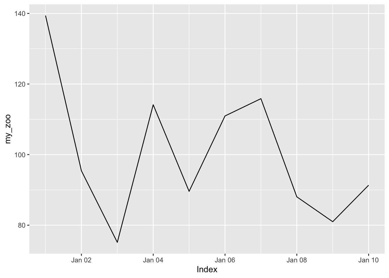

examples

Creating a zoo

zoo objects are an essential tool in the time series analyst tool belt; many advanced functions in time series analysis require time series objects. Creating a zoo object from a vector or data frame is the first step in ensuring your data is ready for a time series analysis!

In this exercise, you’ll create and visualize a time series of the average price of a particular card from a popular trading card game.

You’ll use the core data stored in the vector cards_price, as well as the index vector cards_index, containing the date that each price was sampled.

cards_index, cards_price, and the zoo and ggplot2 packages are available to use.

# Return the head of cards_index
head(cards_index)

[1] "2013-01-01" "2013-01-02" "2013-01-03" "2013-01-04" "2013-01-05"
[6] "2013-01-06"

# Return the head of cards_price
head(cards_price)

[1] 4.88 5.03 5.11 4.77 5.04 5.05

# Create a zoo object: cards_zoo
cards_zoo <- zoo(x = cards_price, order.by = cards_index)

# Autoplot cards_zoo
autoplot(cards_zoo)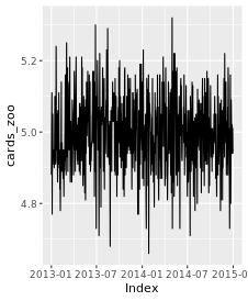

zoo objects, much like data frames, can be visualized with functions from the ggplot2 package. While this course doesn’t go into too much detail regarding ggplot2 plots and functions, it’s nonetheless helpful to review the syntax for more advanced plotting techniques than using autoplot() alone.

In this exercise, you’ll explore using zoo and ggplot2 together. You’ll take the card_prices time series from the previous exercise and generate a ggplot, complete with proper labels, a title, and a theme!

zoo, ggplot2, and card_prices are available to use.

# Enter the x and y axis mapping aesthetics
ggplot(card_prices, aes(x = Index, y = card_prices)) + 
  scale_y_continuous() + 
  # Plot the data with a red-colored line
  geom_line(color = "red") + 

  # Use the light theme
  theme_light() + 

  # Enter the appropriate axis labels and title
  labs(
    x = "Index",
    y = "Price (EUR)",
    title = "Daily Card Prices for Trading Card Game"
  )

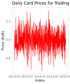
Perfect plotting! ggplot2 has many great options for making an aesthetically pleasing plot, so it’s always a good idea to review some data visualization techniques!

Functions to Manipulate Zoos

zoo objects have two attributes
1. index (time)
- gives the order of observations; allows series to be sorted and compared (instead of relying on raw order)
- observations might not be in proper order if coming from multiple sources; an index ensures each value of each observation is mapped correctly to its time
- creating a zoo from pairs of unsorted values and times will result in an automatically sorted zoo
  - but may not be evenly-spaced, can be large uneven gaps between observations
1. “core data” stored in time series
zoo::index() returns the index attribute (vector of dates)
zoo::coredata() returns the vector of core data

zoo::index(my_zoo)

# replace index
index(my_zoo) <- new_index

zoo::coredata(my_zoo)

# replace core data
coredata(my_zoo)[1] <- 30

Can have overlapping time series, values that occur in more than one dataset

examples

Updating and replacing indices

The data stored in the index of a time series, as well as the core data, can be retrieved and manipulated as a vector in R. While the index attribute is usually a date or time, it can be a vector of unique values of any class, such as character or numeric.

In this exercise, you’ll manipulate the time series coffee_2000s and coffee_2010s, which represent the average daily prices of coffee during the 2000s and 2010s, respectively.

Using lubridate and zoo, you’ll manipulate and update the index of coffee_2000s, which is formatted in a day-month-Year format.

# Assign the index to index_2000s
index_2000s <- index(coffee_2000s)

index_2000s

   [1] "01/01/2000" "01/01/2001" "01/01/2002" "01/01/2003" "01/01/2004"
   [6] "01/01/2005" "01/01/2006" "01/01/2007" "01/01/2008" "01/01/2009"
  [11] "01/02/2000" "01/02/2001" "01/02/2002" "01/02/2003" "01/02/2004" ...

# Parse the day-month-Year index_2000s
index_parsed <- parse_date_time(
  index_2000s,
  orders = '%d/%m/%Y') %>%
  as_date()

index_parsed

   [1] "2000-01-01" "2001-01-01" "2002-01-01" "2003-01-01" "2004-01-01"
   [6] "2005-01-01" "2006-01-01" "2007-01-01" "2008-01-01" "2009-01-01"
  [11] "2000-02-01" "2001-02-01" "2002-02-01" "2003-02-01" "2004-02-01" ...

# Create a zoo based on the new index
coffee_parsed <- zoo(x = coredata(coffee_2000s),
                     order.by = index_parsed)

# Assign the index to index_2000s
index_2000s <- index(coffee_2000s)

# Parse the day-month-Year index_2000s
index_parsed <- parse_date_time(
  index_2000s,
  orders = "%d/%m/%Y") %>%
  as_date()

# Create a zoo based on the new index
coffee_parsed <- zoo(x = coredata(coffee_2000s),
                     order.by = index_parsed)

# Combine the time series and plot the result
coffee_full <- c(coffee_parsed, coffee_2010s)
autoplot(coffee_full)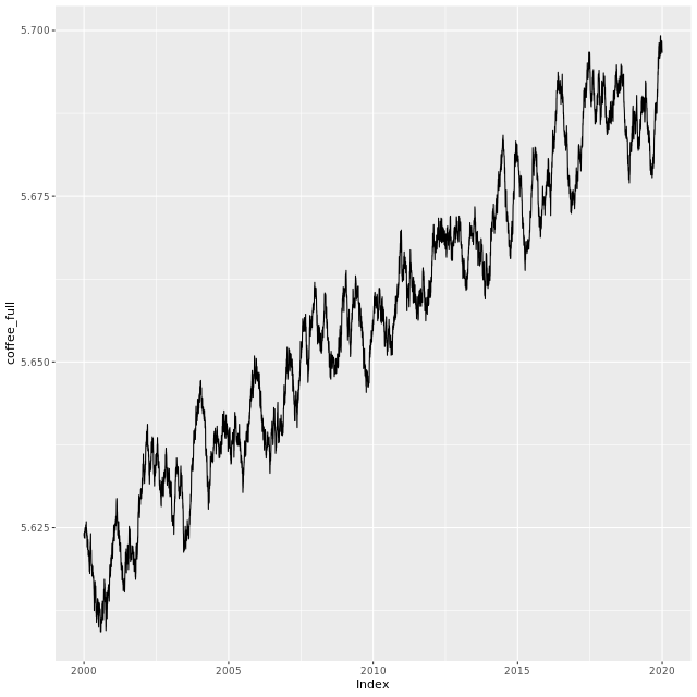

Finding overlapping indices

Time series are said to overlap when there are observations in both time series with the same index, meaning they occur at the same point in time.

By creating a subset using the %in% operator, the overlapping points can be filtered out of one of the time series, allowing the two datasets to be combined.

In this exercise, you’ll take two time series, coffee and coffee_overlap, and remove the elements that overlap.

# Determine the overlapping indexes
overlapping_index <-
  index(coffee_overlap) %in% index(coffee)

# Create a subset of the elements which do not overlap
coffee_subset <- coffee_overlap[!overlapping_index]

# Combine the coffee time series and the new subset
coffee_combined <- c(coffee, coffee_subset)

autoplot(coffee_combined)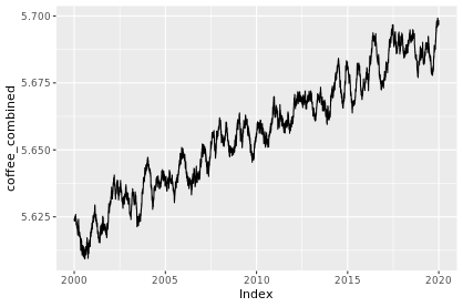

Converting between zoo and dataframe

data.frame
- each variable stored as a column
  - index stored as column, e.g. data$dates
- can’t plot with autoplot
zoo
- each variable stored as a column of a matrix
- index stored as an attribute, e.g. index(data)
- can plot with both ggplot geom and autoplot

Suppose we have a data.frame of prices, to convert to zoo:

prices_zoo <- zoo(x = prices$value,
                  order.by = prices$date)

to convert a zoo to a dataframe:

data_df <- data.frame(index(my_zoo),
                      coredata(my_zoo))

but an even better way, using fortify.zoo():

data_df <- fortify.zoo(my_zoo)

example

When working with real-world time series data, you’ll often import data from spreadsheets and tabular data – data formatted like a data frame. By converting your data to a zoo object, you can be better prepared to perform time series analysis!

Likewise, converting a time series into a data frame allows you to manipulate and export your data in a format that’s widely readable in other software and programming languages outside of R.

The card_prices time series – a time series for the mean daily prices of three trading cards – as well as the lubridate, zoo, and ggplot2 packages have been loaded for you.

card_prices
           price_1 price_2 price_3
2013-01-01    4.88    0.81    2.05
2013-01-02    5.03    0.80    2.11
2013-01-03    5.11    0.82    2.31
2013-01-04    4.77    0.73    2.04
2013-01-05    5.04    0.73    2.03
2013-01-06    5.05    0.73    2.12
2013-01-07    4.94    0.82    2.07
...

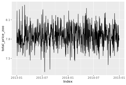
# Fortify to data frame: cards_df
cards_df <- fortify.zoo(card_prices)

# Add together the three price columns from cards_df
cards_df$total_price <-
  cards_df$price_1 +
  cards_df$price_2 +
  cards_df$price_3

# Create the total_price_zoo time series
total_price_zoo <- zoo(x = cards_df$total_price,
                       order.by = cards_df$Index)

# Generate an autoplot of the new time series
autoplot(total_price_zoo)

Time Series in R

Time Series Attributes

Time Series Objects with the zoo package

Functions to Manipulate Zoos

Time Series Objects with the `zoo` package